Introduction to TensorFlow

Introduction

Those who are continuing from the last lesson (Deep Learning) of this series, you might felt deep learning to be a very difficult concept. I agree with you, deep learning is not that easy if you try to implement it from scratch (reinvent the wheel). But in this lesson, we will walk through the final framework in this series, TensorFlow.

Installation

Installing TensorFlow 2 is easy. I will recommend everyone to install TF from pip even if you are using anaconda. Just activate the environment and install TensorFlow with pip. Deep learning algorithms require TPU or GPU to work at a feasible speed. And Tensorflow now natively supports only NVidia graphics cards. NVidia provides API named CUDA and CUDnn for tensor computation which is used by TensorFlow. But these two libraries are required to be installed separately on the machine. pip just installs TensorFlow. But conda can install both TensorFlow with optional CUDA and CUDnn library. In many operating systems (e.g. Linux and Mac), CUDA and CUDnn for conda versions do not work out of the box. That is why I am recommending you to install just TensorFlow with pip, and install CUDA, CUDnn for GPU support.

1
2
3
4
5
6

# pip
pip install tensorflow

# Conda
conda activate <your_env>
pip install tensorflow

But the main difficulty comes when you try to enable GPU support for TensorFlow.

Enable NVidia GPU support for TensorFlow 2

To make TensorFlow compatible with GPU, you need to install CUDA and CUDnn on your machine. Not all versions of CUDA are supported by all versions of TensorFlow. Below is a table for CUDA and TensorFlow 2 compatibility.

Note: If you are familiar with docker, you can just run docker run -it tensorflow/tensorflow bash to get started with TensorFlow with GPU support on any machine.

At the time of writing, the latest version of TensorFlow is 2.5.0. So we will install that version with CUDA 11.2 and cuDNN 8.1.

Here are all the things you need to download first. You may need to create an NVidia developer account to download cuDNN.

1. Latest NVidia GPU driver
2. CUDA-11.2.2
3. cuDNN-8.1

Install the driver and CUDA on your machine. Then extract cuDNN and paste the 3 folders into the directory C:\Program Files\NVIDIA GPU Computing Toolkit\CUDA\v11.2\. If you installed CUDA on another directory, change the path accordingly.

You also need to add a new environment variable named “CUDA_PATH” which will point to “C:\Program Files\NVIDIA GPU Computing Toolkit\CUDA\v11.2”.

For complete guidance on installing cuDNN in different Operating Systems, you may follow the official installation guide

Finally, if you have trouble installing on your machine, or you have a less supported operating system (e.g. Arch Linux, Fedora, etc.), you can follow this guide to install from source.

After installation, test your installation of TensorFlow 2 and GPU support with the following code:

1
2
3
4
5

import tensorflow as tf
if tf.test.is_gpu_available() and tf.test.is_gpu_available(cuda_only=True) and tf.test.is_gpu_available(True, (3,0)):
    print("My GPU supports TensorFlow")
else:
    print("My GPU may be not compatible with TF2")

Tensor Processing in TensorFlow

Tensorflow is built to compute different arithmetics of tensors. In this section, we will start just like we started with NumPy many lessons ago. TensorFlow tries to be as much compatible with NumPy as possible. Although many NumPy features are missing in TensorFlow (like array indexing with array), you will automatically feel at home in TensorFlow if you know NumPy well.

Let’s create a tensor first.

 1
 2
 3
 4
 5
 6
 7
 8
 9
10
11
12
13
14
15
16
17
18
19
20
21
22
23
24
25
26
27
28
29
30

import tensorflow as tf

a = tf.constant([1, 2, 3, 4, 5])
b = tf.convert_to_tensor([6, 7, 8, 9, 10]) # same as above

# All the operations like numpy
print(a + b)
print(a - b)
print(a * b)
print(a / b)
print(a ** b)
print(a & b)
print(a | b)
print(-a)
tf.matmul(a, b)
tf.transpose(a)
tf.exp(a)
tf.log(a)

# It has also many operation methods like NumPy
tf.abs(a) # Absolute
tf.sin(a), tf.cos(a) # Trigonometry

tf.max(a), tf.min(a) # min max
tf.argmax(a), tf.argmin(a)

tf.ceil(a), tf.floor(a), tf.round(a)
tf.sqrt(a)

tf.cumsum(a) # Cumulative Sum

Finally, if you still feel some NumPy features missing in TensorFlow, you can use this snippet to enable NumPy array methods on tensors.

 1
 2
 3
 4
 5
 6
 7
 8
 9
10

print(a.T) # NoAttribute exception

print(tf.transpose(a)) # same functionality

# But I want the a.T notation!!!

from tensorflow.python.ops.numpy_ops import np_config
np_config.enable_numpy_behavior()

print(a.T) # :)

Although all of the snippets above look very similar to NumPy, they are fundamentally very different. The two major differences of tensors and ndarrays are.

1. Tensors are immutable whereas ndarray is mutable.
2. Tensor can be placed on various devices (CPU, GPU, TPU, Ram). But ndarray can only be in CPU.

Placing Tensor on GPU

To compute with GPU, you need to copy the tensors into GPU. To do this, first, make sure your TensorFlow is GPU compatible. And then try to create a tensor with tf.device context manager.

 1
 2
 3
 4
 5
 6
 7
 8
 9
10
11
12
13
14
15
16
17
18

# You need to build a context with TensorFlow to run statements on a specific device.

# Force execution on CPU
print("On CPU:")
with tf.device("CPU:0"):
  x = tf.random.uniform([1000, 1000])
  assert x.device.endswith("CPU:0")
  print(x.shape)
  print('Done')

# Force execution on GPU #0 if available
if tf.config.list_physical_devices("GPU"):
  print("On GPU:")
  with tf.device("GPU:0"): # Or GPU:1 for the 2nd GPU, GPU:2 for the 3rd etc.
    x = tf.random.uniform([1000, 1000])
    assert x.device.endswith("GPU:0")
    print(x.shape)
    print('Done')

Deep Learning with Keras

Keras is a higher-level API built to work with several deep learning libraries like TF, PyTorch, etc. It became so popular that TF2 started to add this Keras with TF backend inside TF2. So now you do not need to install Keras separately. You can access the Keras API with tensorflow.keras.

Keras has two type of API.

1. Sequential API: This API is the simplest one for the deep learning model. Here, everything you declare is an object. You instantiate objects and create a Deep Learning model where the output of one layer is the only output of another layer.
2. Functional API: Keras Sequential API has some limitations. What if you want an output of a layer to be input of two layers? What if you want to concatenate the output of two layers? These are only possible in Functional API.

For this lesson, we will try out the MNIST dataset we used on scikit-learn tutorial. We could use the same load_digit method to load the MNIST dataset with scikit-learn. But TF2 also provides a lot of datasets (more than scikit-learn) to work with. So we will use that dataset in our code.

1
2
3
4
5
6

mnist = tf.keras.datasets.mnist

# The dataset is already split
(x_train, y_train), (x_test, y_test) = mnist.load_data()
x_train, x_test = x_train / 255.0, x_test / 255.0
print(x_train.shape, y_train.shape, x_test.shape, y_test.shape)

Dataset shape conventions in Keras

Datasets that are used for a Keras model always have a specific notation for their shape. The shape should always be like (sample_size, sample_shape...). For example, if the size of an image in a dataset is (28, 28) and there are 100 images for an epoch, then the dataset shape will be (100, 28, 28).

Dataset and Input shape is different most of the time. Dataset shape’s first dimension will contain the total number of samples. And Input’s first dimension will contain the number of samples for each iteration. This number is known as batch size. So the Input shape will be (batch_size, 28, 28).

While defining a model architecture both in Sequential API and Functional API, the batch size is automatically inferred while training. So if you want to create a model, the input size should be only (28, 28).

Keras Sequential API

In Keras, a lot of layers for neural networks are implemented. All we need to do to create a neural network is to instantiate those layers, and create a Sequential Model.

So finally, we will create a model that will take an image as input, and output the SoftMax of 10 classes.

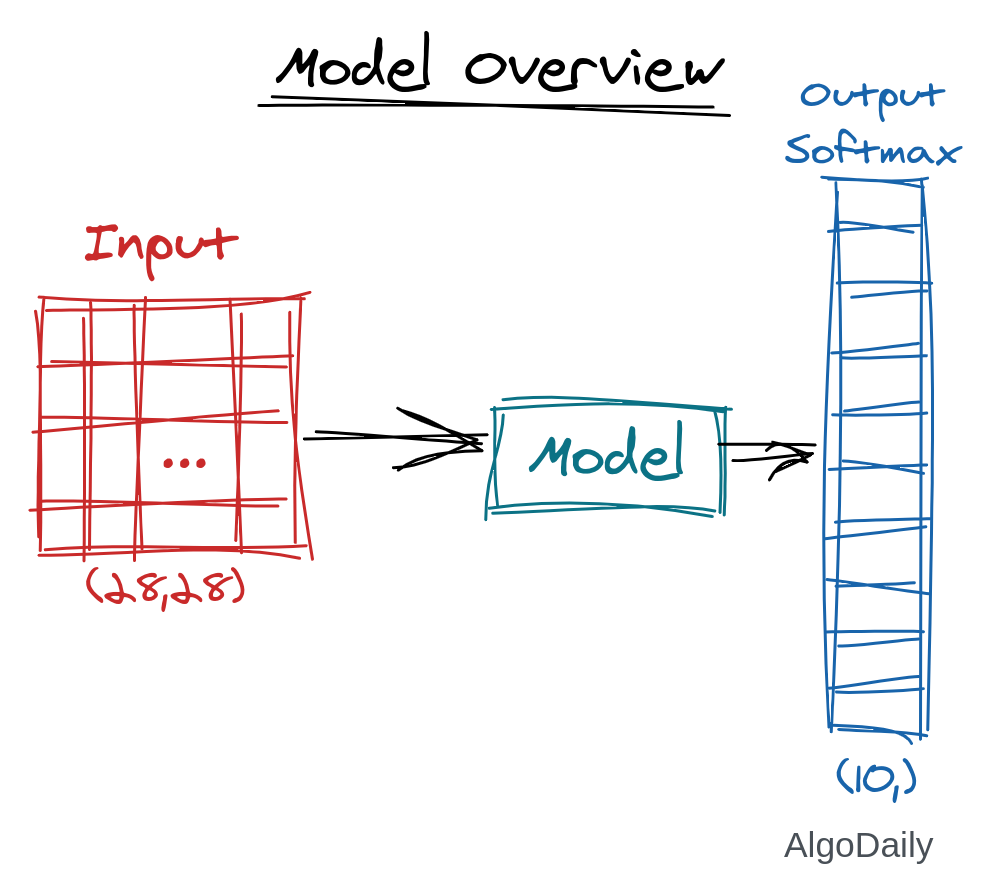
The details of the model are shown in this image:

Here is the code to create a Sequential model in Keras.

 1
 2
 3
 4
 5
 6
 7
 8
 9
10
11

import tensorflow as tf

from tensorflow.keras.layers import Dense, Flatten, Conv2D
from tensorflow.keras import Model

model = tf.keras.models.Sequential([
  tf.keras.layers.Flatten(input_shape=(28, 28)),
  tf.keras.layers.Dense(128, activation='relu'),
  tf.keras.layers.Dropout(0.2),
  tf.keras.layers.Dense(10)
])

Keras Functional API

The same model developed above can again be created with Keras Functional API. You may think that of what the purpose is to create the same model in two different APIS. Honestly, there is no benefit to this exercise. But there are many cases where you cannot create a model using only sequential API. We will just create our digit classification model with Functional API just for the sake of introduction to that API.

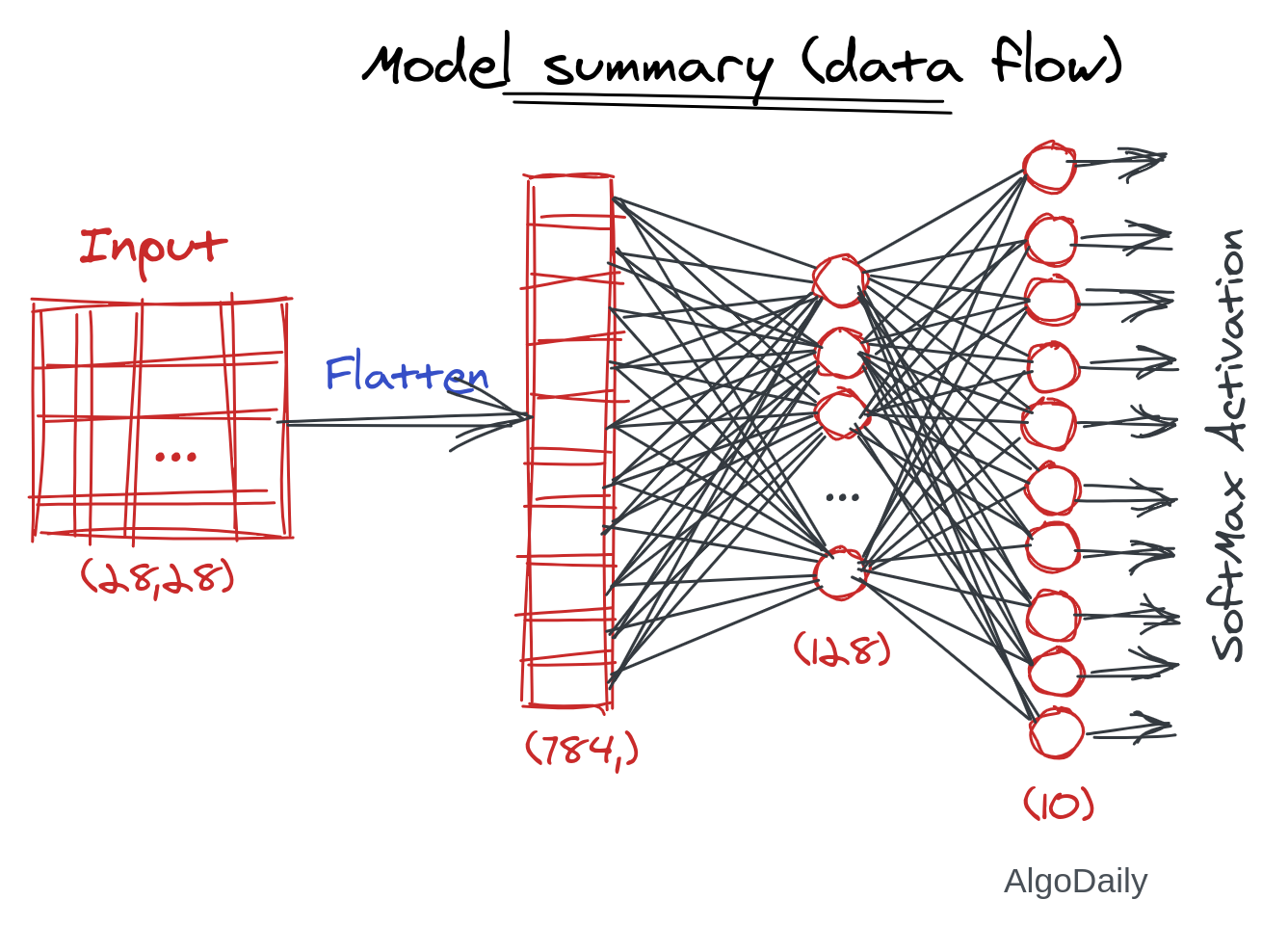
In the previous model, if you think of the data flow in the model, you will have something like the text below:

1
2
3
4
5
6
7
8
9

(input: 784-dimensional vectors)
       ↧
[Dense (64 units, relu activation)]
       ↧
[Dense (64 units, relu activation)]
       ↧
[Dense (10 units, softmax activation)]
       ↧
(output: logits of a probability distribution over 10 classes)

The functional API works more closely to the data flow than the model architecture. You input a data placeholder into a model, and you will get an output placeholder. You can use that output as an input to other layer instances. Let’s see that in action.

First, we have to instantiate all the layers we need in the model. The layers are not connected to each other in this step.

1
2
3
4
5

# Instantiating the layers. These layers are not connected to each other.
flatten = tf.keras.layers.Flatten()
dense1 = tf.keras.layers.Dense(128, activation='relu')
dropout = tf.keras.layers.Dropout(0.2)
dense2 = tf.keras.layers.Dense(10, activation='softmax')

Then we create an Input placeholder. The shape of the MNIST dataset is (28, 28). You can verify this by seeing x_train.shape.

1

inputs = keras.Input(shape=(28,28))

The final part is to connect all the layers we created so far given a flow of data into those layers. We pass the inputs as a parameter to our first layer and get a return value. Let’s call it x. Then we pass this x to the new layer and get another return value. We will continue this to the last layer. The output of the final layer is the actual output of our model (after activation function).

1
2
3
4
5

inputs = tf.keras.Input(shape=(28,28))
x = flatten(inputs)
x = dense1(x)
x = dropout(x)
outputs = dense2(x)

But like the Sequential API, we do not have any model object. tf.keras.Model objects help you to use a single object to train, modify and predict from different datasets. We can use the constructor of Model to create one. In that model, two parameters are needed. The inputs placeholder, and the outputs placeholder. We can also provide a name for the model.

1

model = tf.keras.Model(inputs=inputs, outputs=outputs, name="mnist_model")

It is always a good practice to create a model inside a function. Then we can create as many models as we want by simply calling that function.

 1
 2
 3
 4
 5
 6
 7
 8
 9
10
11
12
13
14
15
16
17

def get_model():
    # Instantiating the layers. These layers are not connected to each other.
    flatten = tf.keras.layers.Flatten()
    dense1 = tf.keras.layers.Dense(128, activation='relu')
    dropout = tf.keras.layers.Dropout(0.2)
    dense2 = tf.keras.layers.Dense(10, activation='softmax')
    
    inputs = tf.keras.Input(shape=(28,28))
    x = flatten(inputs)
    x = dense1(x)
    x = dropout(x)
    outputs = dense2(x)
    
    model = tf.keras.Model(inputs=inputs, outputs=outputs, name="mnist_model")
    return model

model = get_model() 

To see the details of a model, you can use model.summary() which will print all the layers with their output shape, and the number of parameters to train.

 1
 2
 3
 4
 5
 6
 7
 8
 9
10
11
12
13
14
15
16
17
18
19
20

model.summary()

Model: "mnist_model"
_________________________________________________________________
Layer (type)                 Output Shape              Param #   
=================================================================
input_8 (InputLayer)         [(None, 28, 28)]          0         
_________________________________________________________________
flatten_9 (Flatten)          (None, 784)               0         
_________________________________________________________________
dense_18 (Dense)             (None, 128)               100480    
_________________________________________________________________
dropout_9 (Dropout)          (None, 128)               0         
_________________________________________________________________
dense_19 (Dense)             (None, 10)                1290      
=================================================================
Total params: 101,770
Trainable params: 101,770
Non-trainable params: 0
_________________________________________________________________

Loss functions with Keras

Keras has a lot of loss functions defined inside the tf.keras.losses submodule. As the output is of 10 classes, we will need SparseCategoricalCrossentropy loss function. We can instantiate one like below:

1
2
3
4
5
6

loss_fn = tf.keras.losses.SparseCategoricalCrossentropy(from_logits=False)

# For test, the loss_fn can be used like this:
y_true = [1,2]
y_pred = [[0.05, 0.95, 0], [0.1, 0.8, 0.1]]
loss_fn(y_true, y_pred)

Optimizer in Keras

Optimizer is a new word to you till now. Until now, we used a loop to go through the iterations and epochs of the training process. Tensorflow has scikit-learn like .fit and .predict method, so you do not need to explicitly run a loop. Moreover, you do not need to calculate the gradient by yourself or apply the gradient to update the trainable parameters (of course you can do that by yourself). This requires the mathematical knowledge behind the gradient descent algorithms as we did in the last lessons. Also, there are many variants of gradient descent algorithms like Adam, Adadelta, Adagrad, RMSProp, and many more. We have to understand the mathematics behind all of these algorithms to implement them in code.

But TensorFlow has overcome this procedure by introducing tf.keras.optimizers. By default, TensorFlow maintains a graph of calculations of different tensors. That graph has all the tensors as edges and all the operations as nodes. When an operation is done on a tensor, the gradient of the tensor is automatically calculated behind the scene. So, in the backpropagation process, all one needs to do is use learning rate and other algorithms specific parameters to apply that gradient descent algorithm to update weights.

All of these are done using an Optimizer object. Optimizers in TensorFlow take the necessary parameters for that weight optimization algorithm and runs the given number of iterations for you. Let us use the well-established Adam optimizer for now. Check out the link for all other optimization algorithms and how they work as well.

1

optimizer = tf.keras.optimizers.Adam(learning_rate=0.001)

Model Compilation

Now we have all the ingredients to start the training process. We can just call model.fit(x_train, y_train) to start the training! But wait, how would the model know that we will use our initialized Adam optimizer and the loss_fn loss function for the training? We need to link our model with those optimizers and loss functions.

Moreover, while training, we want to watch the loss go down live. Or we may want to see the accuracy increase at each epoch. All these are known as metric. We can optionally provide a metric to our model at compilation to watch it while training.

1
2
3
4
5

model.compile(
    optimizer=optimizer,
    loss=loss_fn,
    metrics=['accuracy']
)

Training loop

As stated earlier, we do not need to explicitly run a loop for the training. The optimizer will handle it for us. Like scikit-learn, we can run model.fit to see the training live.

1

model.fit(x_train, y_train, epochs=5)

Model evaluation

To see how good our model is on the cross-validation set, we can run an evaluation of our model on the cross-validation set.

1

model.evaluate(x_test,  y_test)

We can also predict new datasets using the trained model. If we have a new dataset names x_test_new, we can get y_pred using the predict method.

1

y_pred = model.predict(y_test_new)

Callback functions, Checkpoint, saving and loading model

Training a large neural network is a long time process. Many current neural networks even take weeks to fully train. Imagine you are training a model, but almost at the end of the training, you have a power-cut or some other problem. You will need to retrain the whole model again. The training of the model can be saved at different points using a ModelCheckpoint callable callback object.

While training a model, TensorFlow provides a way to call any callable (functions, classes, etc.) at each epoch. TF2 also provides a lot of already implemented callables. You can use those callables by passing them to the .fit method. In the below snippet, we will use the tf.keras.callbacks.ModelCheckpoint callback to save the model at each epoch if the metric is higher than the current save.

1
2
3
4
5
6

model_checkpoint_callback = tf.keras.callbacks.ModelCheckpoint(
    filepath='checkpoint/',
    save_weights_only=True,
    monitor='accuracy',
    mode='max',
    save_best_only=True)

Then we can pass this callback while training the model.

1

model.fit(x_train, y_train, epochs=5, callbacks=[model_checkpoint_callback])

If you want to resume the training on a new machine after an interruption, just load the model weights before training.

1

model.load_weights('checkpoint/')

While training the model, you will find a new folder named checkpoint where the model with the best accuracy will be saved.

After training the model, you can save and load the model object to a file and share that with anyone. For this, you need to install some dependency libraries. Install them with the following commands:

1

pip install -q pyyaml h5py

Now use this snippet to save and load model

1
2
3
4
5

# Save the model
model.save('saved_model/my_model')

# Load the model
model = tf.keras.models.load_model('saved_model/my_model')

Conclusion

In this lesson, we have gone through all the fundamentals of TensorFlow 2. But honestly, we just scratched the surface. TensorFlow library is huge. It is used both by many researchers in Academia and by many real-life programmers for production-ready software. Now that you can load and preprocess the dataset, build a model, train a model and finally save the model; go ahead and look for some dataset online. Then train a new model on that dataset and see what the results are. In another lesson, we will discuss how to effectively find a dataset and cite that dataset in your ML model. We will soon also look at many popular machine learning algorithms like CNN, LSTM, and many established models (e.g. Yolo, R-CNN, GPT3, etc.). Until then, make sure you are very comfortable working with TensorFlow.