All about Numpy and Pandas

Introduction

NumPy and Pandas are the most popular libraries for numeric computation in python. NumPy is so popular that there are debates that the library should be built into python itself and not a separate module. In this lesson, we will walk through many useful features that these two giant libraries offer. After this lesson, you will be very comfortable with both of these libraries.

NumPy’s calculative protocols are so popular that, popular Machine Learning frameworks like TensorFlow and PyTorch follow this protocol into their own tensor computation. They also provide methods to retrieve tensors as NumPy arrays. So learning this will help you to use almost all other advanced modules we will introduce in future lessons. Finally, in your upcoming Machine Learning career, you will never have trouble using these two libraries.

Basics of Matrix

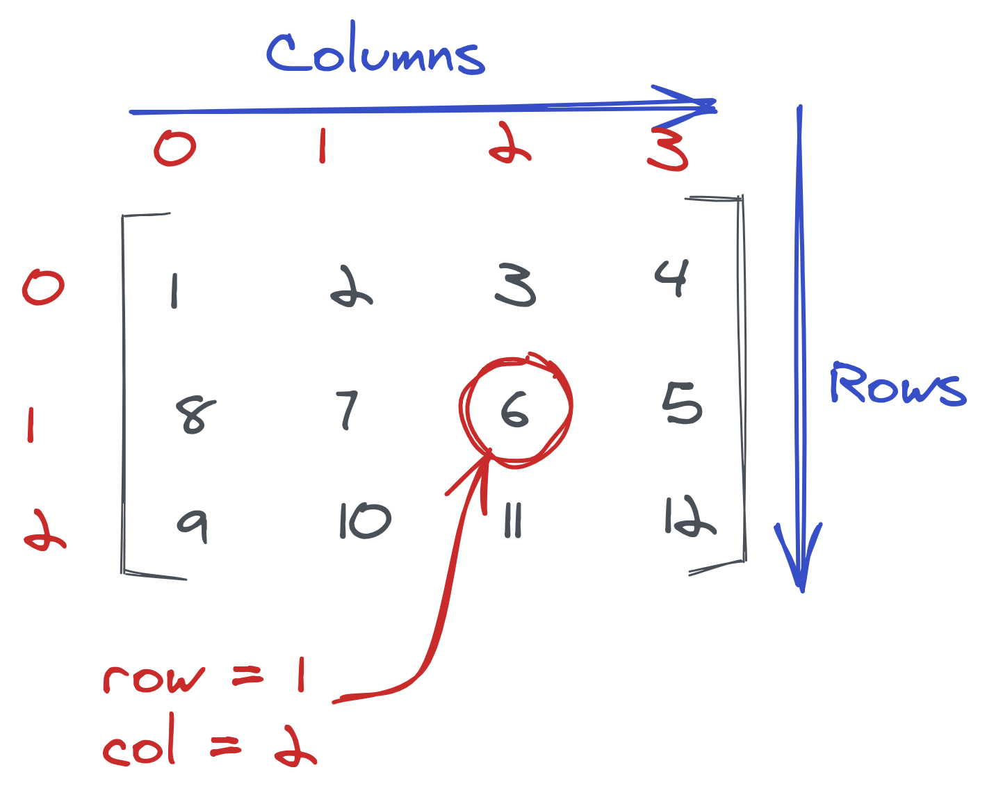
Before manipulating data in NumPy, you need some fundamental knowledge of matrix. A matrix is a collection of numbers arranged into a fixed number of rows and columns. It can also be thought of as a grid of numbers. Below is an example of a matrix:

In python, you can define a matrix using a two-dimensional list. We will go through dimensionality later in this lesson, but for now, think of a two-dimensional list as a list within a list. See the above matrix implemented in python below:

1
2
3
4
5
6
7
8
9

a_matrix = [
    [1,  2,  3,  4],
    [8,  7,  6,  5], 
    [9, 10, 11, 12]
]

# Accessing elements

print(a_matrix[1][2]) # 6

Remember, a matrix should always have equal rows in all columns, and equal columns in all rows. b_matrix in code below is not a matrix:

1
2
3
4
5
6

# not a matrix
b_matrix = [
    [1,  2,  3,  4],
    [8,  6,  5],  # This row has 3 columns and the rest has 4
    [9, 10, 11, 12]
]

Operations in Matrix

Addition and subtraction

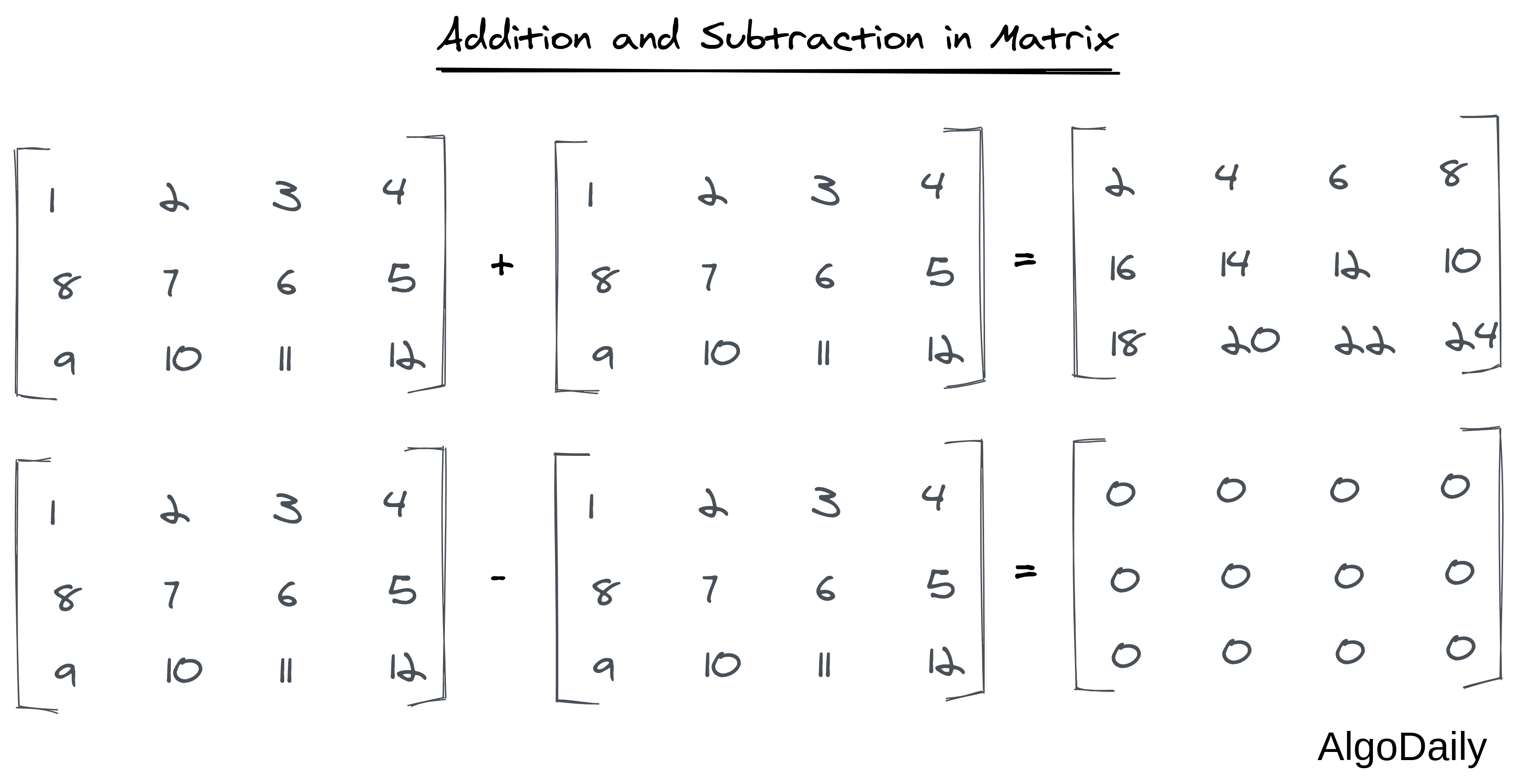
Addition and subtraction in matrices are always element-wise. See an example below:

In python, it can be implemented by the code:

1
2
3
4
5
6
7
8

def addition(mat_a, mat_b):
    mat_c = []
    for row_a, row_b in zip(mat_a, mat_b):
        row_c = []
        for col_a, col_b in zip(row_a, row_b):
            row_c.append(col_a+col_b)
        mat_c.append(row_c)
    return mat_c

Multiplication in Matrix

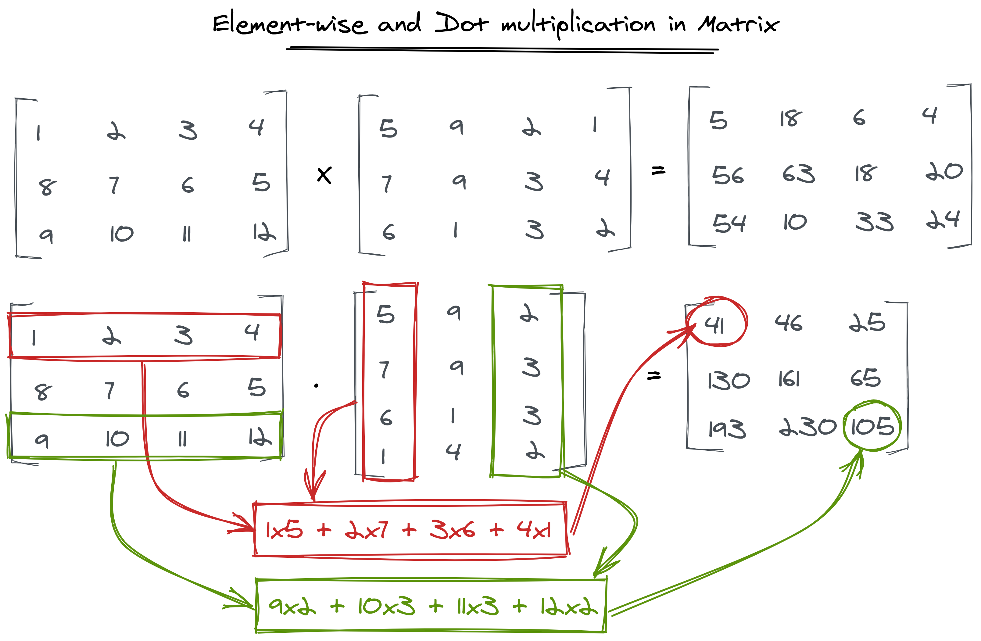
There are two types of multiplication in matrices. Dot multiplication and element-wise multiplication. Element-wise multiplication is self-describing. We multiply each element of the two matrices just like addition/subtraction.

But dot multiplication is a little tricky. In dot multiplication, each element will be the sum of all the rows of the first matrix element-wise multiplied by all the columns of the second matrix one by one.

See the image below to understand both multiplications.

Shape of Matrix

The shape of a matrix is a feature that defines the structure of the matrix. The shape of a matrix is number of rows x number of columns. So the matrices used in the addition/subtraction section are of shape 3x4. In python, shapes are defined as tuples. So the shape of that matrix is (3, 4). We will understand this more in a bit when we start working with NumPy.

Tensor

Tensors are the core knowledge about data to use in Data Science. They are a more generalized form of Matrices. A tensor can be a single number or can be a more complex data structure than a matrix. According to Wikipedia:

In mathematics, a tensor is an algebraic object that describes a (multilinear) relationship between sets of algebraic objects related to a vector space.

Although this definition is a lot to digest, tensors aren’t actually that difficult to understand. The reason I introduced matrices before tensors are to make tensors more understandable. Think of tensors as blocks of data.

Let us start with a single number. This tensor has only 1 dimension (because it can be counted in only 1 way). And the shape will consist of only 1 integer (because of 1 dimension). How many values are there when counted in the first way? Only 1! So the shape will be (1,) in python tuple notation.

Now let’s increase the numbers count in the tensor. This tensor can also be counted in one way only (from left to right, or top to bottom if you write it in that way). So the dimension would be one. This first dimension is said to be dimension number 1. In this first dimension, there is a total of 5 values. So the shape of this tensor will be (5,).

Let’s increase those number count even more. But this time, we will increase the number in another direction. So a new dimension to the tensor will be added. And now the tensor can be counted in 2 directions. First, we can count the rows, and then count the columns (or vice-versa). So the dimension of this tensor will be 2. Typically, the rows are counted first, and then the columns. So the shape of the tensor will be (3, 5) because we will get 3 rows on the first dimension and 5 columns on the second dimension. Note that, this is exactly like a matrix. A matrix is nothing but a 2D tensor.

Finally, we can enlarge the tensor even more to a new dimension. This tensor will have 3 dimensions and the shape will be (3, 5, 3). First, we will have 3 planes when counting from left to right. Then in each plane, we have matrices of shape (5,3).

If you try to increase the dimension even more (create a 4D or 5D tensor), things will start to become difficult to imagine. But you can take 3 of the above 3D tensors side-by-side, and think of the whole picture as a 4D tensor.

Operations in tensor are the same as matrices discussed in the previous section. We do element-wise addition, subtraction, and multiplication. There is also a way to do dot products of two multidimensional tensors, but we are leaving this for later as it is too complex for the score of this series. Now let us see how to handle tensors in NumPy.

NumPy

Although NumPy calls tensors just arrays, they do all the operations among those like tensors. NumPy has a scalar type for a single value and ndarray type for tensors. To create an ndarray directly in code, you can create a list in python first, then call np.array(). Look at the below code:

 1
 2
 3
 4
 5
 6
 7
 8
 9
10
11
12
13
14
15
16
17
18
19

import numpy as np

tensor_list = [
    [
        [1, 2, 3],
        [4, 5, 6],
        [7, 8, 9]
    ],
    [
        [11, 12, 13],
        [14, 15, 16],
        [17, 18, 19]
    ],
]

tensor = np.array(tensor_list)

print('Shape is :', tensor.shape) # (2,3,3)
print('Dimension is :', len(tensor.shape)) # 3

NumPy has a lot of convenient functions to create ndarrays. Look at the the code snippet below to understand some basic functions like these:

 1
 2
 3
 4
 5
 6
 7
 8
 9
10
11
12
13
14
15

a = np.ones([2, 2, 3]) # A tensor of shape (2, 2, 3) with all ones
# Use the above function to create a tensor with given shape filled with any value
a2 = np.ones([2, 2, 3]) * 5 # A tensor of shape (2, 2, 3) with all 5s
a3 = np.full([2, 2, 3], 5) # Same and better than above

b = np.zeros([2, 2, 3]) # A tensor of shape (2, 2, 3) with all zeros

c = np.arange(10) # A tensor of shape (10,) populated with 0..9
d = c.reshape([2, 5]) # A tensor of shape (2, 5) populated with 0..9 (row first)

e = np.empty([2, 2, 3]) # This function is the fastest. Because it just captures the memory and does not initialize it. So there will be garbage values in this tensor

f = np.eye(4, 4) # Identity matrix with 1 in diagonal and 0s elsewhere. 

g = np.linspace(0, 10, 5) # A tensor of shape (5,) initialized with equidistant values from 0 to 10

Other than the functions above, you can also create ndarrays with the random submodule of NumPy. We will look at it soon.

Operations in NumPy

The most pleasing thing about NumPy is its operations’ simplicity. We will discuss some major kinds of operations here:

Arithmetic Operations

Numpy does operations on tensors just like python does operations on its primitive types. The only constraint here is that the arrays must be of the same shape. There is an exception to this which we will cover in the next section of broadcasting. Run the code below and see the example results yourself.

 1
 2
 3
 4
 5
 6
 7
 8
 9
10
11
12
13
14
15
16

a = np.array([
    [1, 2, 3],
    [2, 3, 4]
])
b = np.array([
    [6, 7, 8],
    [7, 8, 9]
])

print(a + b) # Element-wise addition
print(a - b) # Element-wise subtraction
print(a * b) # Element-wise multiplication
print(a / b) # Element-wise division
print(a // b) # Element-wise integer division
print(np.dot(a, b)) # Matrix dot product. This will not work as shapes do to match
print(np.dot(a, b.T)) # Transpose b, then dot product

Tensor/Array Slicing

One of the most powerful features of NumPy is its tensor slicing. You can slice a tensor in any dimension very efficiently. It is just like list slicing in python. The only difference is that you need to indicate the slicing range in each dimension from the first. Think of these as lists that you are slicing in python. In the example below, take a closer look at the output shape of the arrays after slicing.

 1
 2
 3
 4
 5
 6
 7
 8
 9
10
11
12
13
14
15
16
17
18
19
20

a = np.array([
    [
        [1, 2, 3],
        [4, 5, 6],
        [7, 8, 9]
    ],
    [
        [11, 12, 13],
        [14, 15, 16],
        [17, 18, 19]
    ],
])

print(a)           # (2, 3, 3)
print(a[0])        # (3, 3)
print(a[0][1])     # (3,)
print(a[0, 1])     # (3,) Same as above
print(a[:1, 1])    # (1, 3)
print(a[:1, :])    # (1, 3, 3)
print(a[:1, :, 2]) # (1, 3)

As a rule of thumb, always think of the slicing indices paired with their corresponding dimensions. The first index will cut the array in the first dimension. The second one will cut the array in the second dimension. If you don’t provide slicing indices in all the dimensions, NumPy will think that you are putting : for those. And if you want to take all the elements in an earlier dimension and slice in a later dimension, you can explicitly do that using : as I did in the last print statement of the example above.

Broadcasting in NumPy

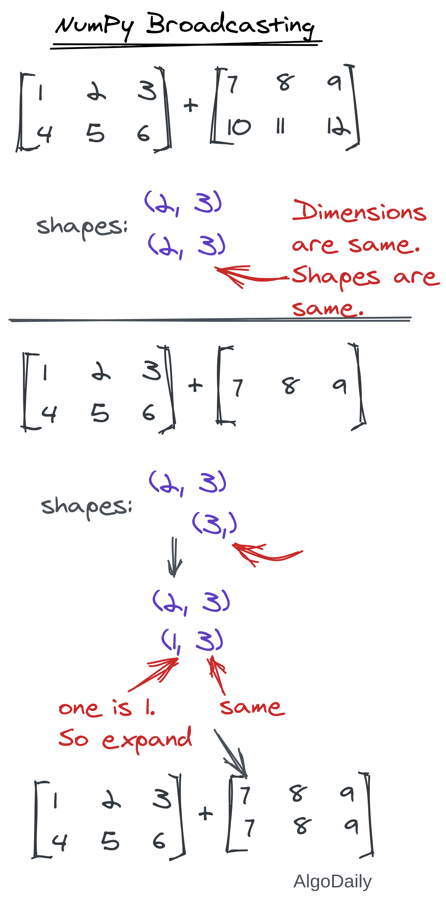
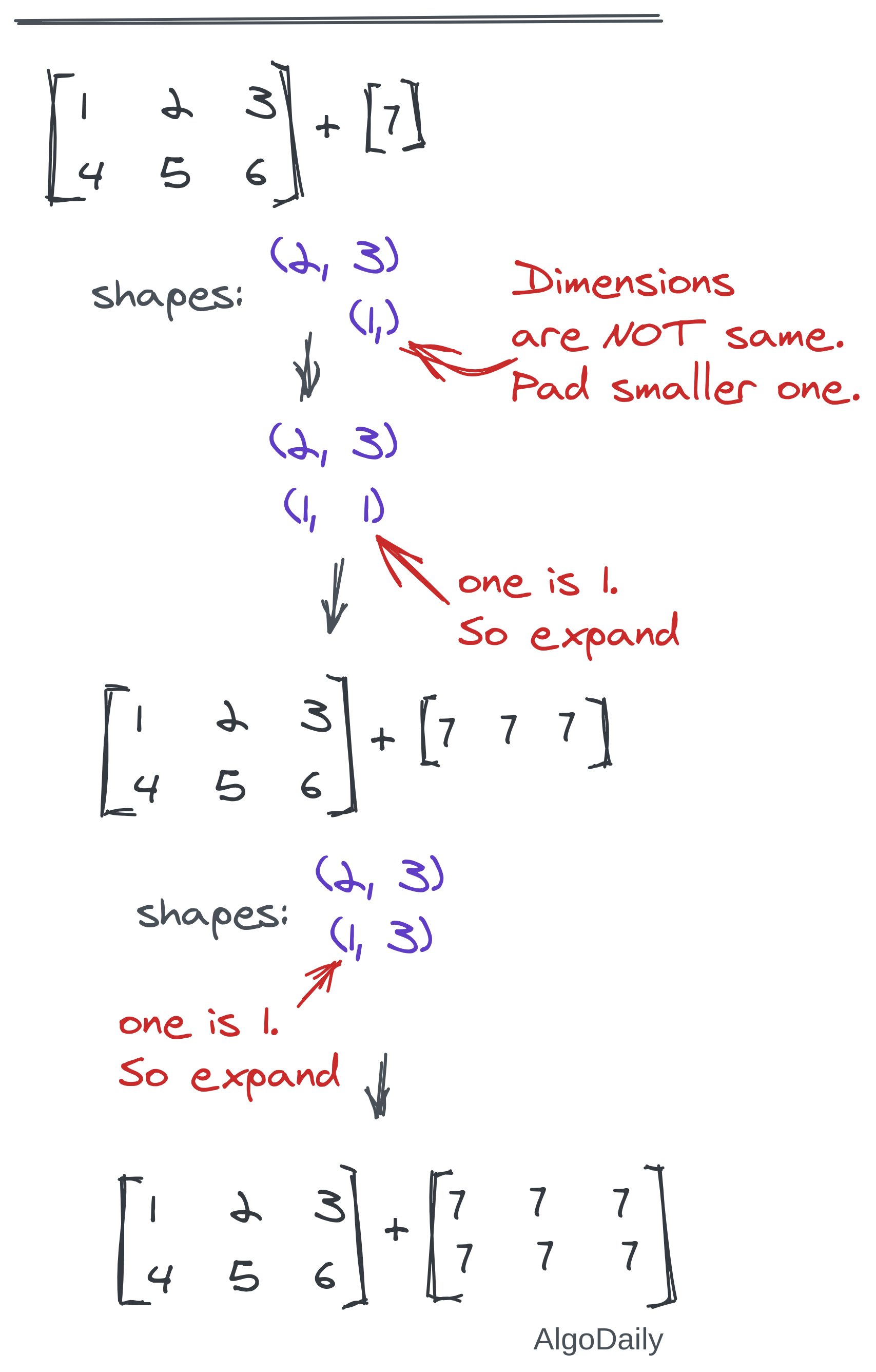
This is the most difficult concept in this easy NumPy world. Broadcasting allows you to make operations among two tensors of different shapes. Whenever a dimension is found to be 1 in one of the ndarrays, NumPy automatically broadcasts that dimension to match the shape of two tensors. All you need to remember is the following two rules one of which must be satisfied for operations between two NumPy arrays:

1. The size of the corresponding dimensions must be the same.
2. The size of one of the corresponding dimensions is 1.

If the dimensions of two arrays are not the same, the dimension of the smaller array is padded on the left with ones to fulfill the requirements. Let us go through some examples in the image below:

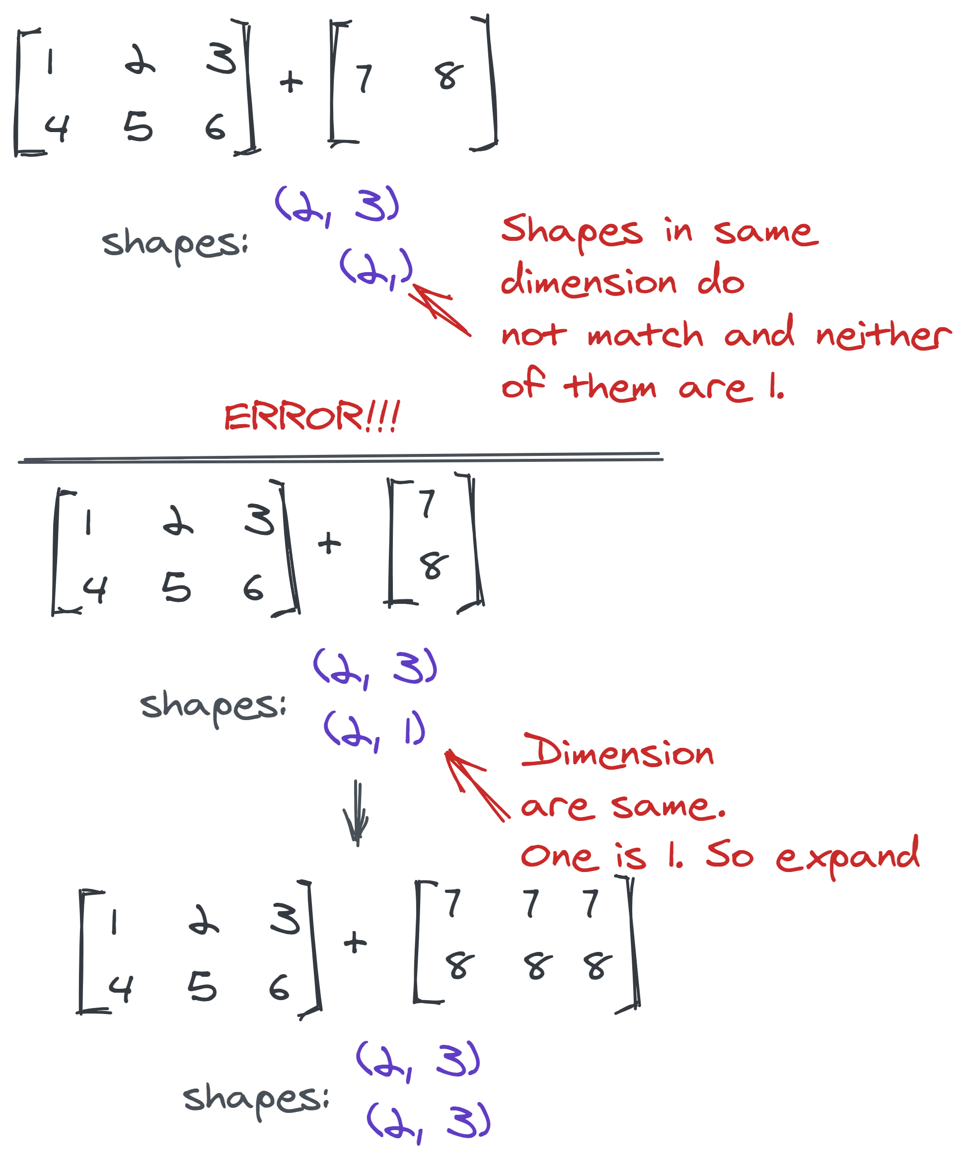
A more confusion clearing demonstration is given below:

Pandas

Pandas is much similar to NumPy, but are much more focused on tabular data. Unlike ndarrays, it has Series (1D array) and DataFrame (2D array). Another advantage of using pandas is its manageability for large data. Pandas can easily manage 50,000 rows or more, and it can work on that data chunk by chunk. It also consumes larger memory than NumPy. The best place where you want to use pandas over numpy is where you need to work with CSV files or any other tabular data instead of multidimensional arrays.

We have already installed pandas library in the previous lesson in the newenv conda environment. Let us see how we can use it in our code. We will load a CSV file from the internet into memory with pandas.

 1
 2
 3
 4
 5
 6
 7
 8
 9
10
11
12
13
14

import pandas as pd

df = pd.read_csv("https://datahub.io/machine-learning/iris/r/iris.csv")

#%% # This comment means you should start a new jupyter notebook cell from here

df.head(5) # Shows first 5 rows

#%%
df.tail(5) # Shows last 5 rows

#%%
# If you are not using an interactive jupyter notebook, you can use this to_string() method in terminal
print(df.head().to_string())

Pandas can be used to analyze, clean, explore, and manipulate data. The main two types in pandas are DataFrame and Series. A Series will always have a fixed datatype, but a dataframe can have many Series with different datatypes. We have already created a dataframe from a CSV URL. Let us see how we can create these two objects directly in code:

 1
 2
 3
 4
 5
 6
 7
 8
 9
10
11
12
13
14
15
16
17
18
19

df = pd.DataFrame({
    'column 1': [1, 2, 3, 4],
    'column 2': ['box', 'car', 'juice', 'chair'],
})
df

#%%
ser = pd.Series([
    'a', 'b', 'c', 'd'
], index=['col 1', 'col 2', 'col 3', 'col 4'])
ser

#%%
# Accessing a column in dataframe will return a Series
df['column 1']

#%%
# Accessing a column in Series will return the actual value
ser['col 1']

This is all that is new about pandas to you! You can now to do all sorts of things that you could do with numpy. You can slice indices of a dataframe or Series or do operations among columns of two DataFrames.

1
2
3
4
5
6
7
8
9

# Accessing rows
df.loc[0] # First row
df.loc['column 1'] # row by name
df.loc[[0,1]] # First two rows
df.loc[:10] # First 10 rows

# Accessing columns
df.loc[:10]['columns 1'] # First 10 rows and column 1 as series
df.loc[:10]['columns 1'][1] # First 10 rows and column 1s second value

Besides reading CSV files with read_csv function, pandas can also read and write a dataframe into different types of files like JSON, CSV, xlsx, etc.

 1
 2
 3
 4
 5
 6
 7
 8
 9
10
11
12
13
14
15
16
17
18
19
20
21
22
23

# json
df = pd.read_json('data.json')
df.to_json('data.json')

#%%
# csv
df = pd.read_csv('data.csv')
df.to_csv('data.csv')

#%%
# Excel
df = pd.read_excel('data.xlsx')
df.to_excel('data.xlsx')

#%%
# HTML
df = pd.read_html('data.html')
df.to_html('data.html')

#%%
# Pickle
df = pd.read_pickle('data.pickle')
df.to_pickle('data.pickle')

Finally, we will cover the most powerful method in pandas. The apply method. This method can be used to apply a function to any column or row in a dataframe. That function should receive a Series as an argument and return a value or Series. Depending on the value or series, a new Series or dataframe will be returned from apply after applying the function to that row or column. See the example below:

 1
 2
 3
 4
 5
 6
 7
 8
 9
10
11
12
13
14
15
16
17
18
19
20
21

import pandas as pd

df = pd.read_csv("https://datahub.io/machine-learning/iris/r/iris.csv")

#%%
def add_first_and_second_column(row):
    return row[0] + row[1]

df['col0 + col1'] = df.apply(all_first_and_second_column, axis=1)
df

#%%
# You can also use lambdas quickly
df['col0 + col1'] = df.apply(lambda row: row[0] + row[1], axis=1)
df

#%%
# This operation is just adding two columns, 
# So we can also do this without using apply
# But many operations WILL need to use apply
df['col0 + col1'] = df[0] + df[1]

Columns will be passed to the function when axis=0 and rows will be passed when axis=1. Finally, if your data is too large, you can get a brief description of it using the df.describe() method.

Conclusion

You are now a growing data scientist who knows his way around a dataset. You can now load data into memory, analyze and process the data in any way you want. Check out the documentation for both NumPy and Pandas. Then download a bunch of CSV and NumPy (np) files from online and play with them. In a later lesson, we will give you a guide on how to search and download a dataset more efficiently. Till then, keep patience and continue learning with me throughout this series.