Into the world of Machine Learning

Introduction

In this lesson, we will build our first Machine Learning algorithm with only Numpy. We will make you understand what machine learning really is. By this lesson, you will understand many types of classes and common keywords in Machine Learning.

Intuition

Let us first build a program that will try to guess a number you imagined by simply correcting the output of the program. The computer will try to guess a number and show it to you. Then you will tell the computer that the number is bigger or smaller than your guessed number. After that computer will guess again and show it to you. By iterating over this for long enough, you’ll see that the computer will slowly become accurate. Let us build the program step by step.

First, the computer will guess a number. We can easily do this using the random built-in module in python. Let us think that the number will be always between 0 and 100. We will also keep track of how many retries the computer had to do to guess my number correctly. It will start from 0.

1
2
3
4

import random

guess = random.randint(0, 100)
tries = 0

Now we will build the skeleton of the program. The computer will keep guessing until the guess is close enough. So we can do an infinite loop and ask the user when the guess is close enough to stop the loop. We also need to know whether the guess is bigger or smaller if it is not close enough.

 1
 2
 3
 4
 5
 6
 7
 8
 9
10
11
12
13
14
15
16
17
18
19
20
21
22
23
24
25
26
27
28
29
30

import random

guess = random.randint(0, 100)
tries = 0

# This is known as the training loop in ML. Because we are updating our parameter "guess" in this loop
while True:
    tries += 1
    print("My guess is :", guess)
    print('''Is the guess close enough?
    1: Yes!!
    2: The guess is bigger
    3: The guess is smaller

        : 
    ''', end='')
    comp = int(input())
    # Input validation
    if comp not in [1, 2, 3]:
        print("Input is invalid")
        continue
    
    if comp == 1:
        print("I did it!!!")
        print("Total tries needed :", tries)
        break
    elif comp == 2:
        # Decrement guess
    elif comp == 3:
        # Increment guess

We only need the logic part of updating the guess to complete the program. We could simply increment/decrement guess by one. But this would be very tedious and the computer will need a lot of retries. So what we can do is increment the guess by a bigger value. Let’s call it jump (the guess is jumping towards the answer).

1
2
3
4
5
6
7

jump = 20

# in decrement part
guess -= jump

# in increment part
guess += jump

But if we keep the jump fixed, do you see what went wrong during the play? The guess never comes close to the actual answer. So we somehow need to decrement the value of jump throughout the iterations. But what if we need to jump only in a positive direction to get to the result. In that case, no need to decrease the jump length as it will only slow the convergence process.

So what can we do here? The solution is that we keep track of the jump direction. If the jump direction changes, we know that we accidentally jumped too far. So we need to jump in the other direction a little smaller. Let’s do it in the code.

 1
 2
 3
 4
 5
 6
 7
 8
 9
10
11
12
13
14
15
16
17
18
19
20
21
22
23
24
25
26
27
28
29
30
31
32
33
34
35
36
37
38
39

import random

guess = random.randint(0, 100)
tries = 0
jump = 20
last_comp = 0 # Keeping track of the direction
decrement_jump = 2

while True:
    # 80
    tries += 1
    print("My guess is :", guess)
    print('''
    
    Is the guess close enough?
    1: Yes!!
    2: The guess is bigger
    3: The guess is smaller

        : ''', end='')
    comp = int(input())
    if comp not in [1, 2, 3]:
        print("Input is invalid")
        continue
    
    # Oops, we jumped too far. So decrement jump
    if last_comp != comp:
        jump /= decrement_jump
            
    if comp == 1:
        print("I did it!!!")
        print("Total tries needed :", tries)
        break
    elif comp == 2:
        guess -= jump
    elif comp == 3:
        guess += jump
        
    last_comp = comp

The program is now complete. Run it and the computer should be able to guess your answer after some retries like below where I guessed 20:

  1
  2
  3
  4
  5
  6
  7
  8
  9
 10
 11
 12
 13
 14
 15
 16
 17
 18
 19
 20
 21
 22
 23
 24
 25
 26
 27
 28
 29
 30
 31
 32
 33
 34
 35
 36
 37
 38
 39
 40
 41
 42
 43
 44
 45
 46
 47
 48
 49
 50
 51
 52
 53
 54
 55
 56
 57
 58
 59
 60
 61
 62
 63
 64
 65
 66
 67
 68
 69
 70
 71
 72
 73
 74
 75
 76
 77
 78
 79
 80
 81
 82
 83
 84
 85
 86
 87
 88
 89
 90
 91
 92
 93
 94
 95
 96
 97
 98
 99
100
101
102
103
104
105
106
107
108
109
110
111
112
113
114
115
116
117
118
119
120
121
122
123
124
125
126
127
128
129
130
131
132
133
134
135
136
137
138
139
140
141
142

My guess is: 99
Is the guess close enough?
    1: Yes!!
    2: The guess is bigger
    3: The guess is smaller

        : 2
My guess is : 89.0
Is the guess close enough?
    1: Yes!!
    2: The guess is bigger
    3: The guess is smaller

        : 2
My guess is : 79.0
Is the guess close enough?
    1: Yes!!
    2: The guess is bigger
    3: The guess is smaller

        : 2
My guess is : 69.0
Is the guess close enough?
    1: Yes!!
    2: The guess is bigger
    3: The guess is smaller

        : 2
My guess is : 59.0
Is the guess close enough?
    1: Yes!!
    2: The guess is bigger
    3: The guess is smaller

        : 2
My guess is : 49.0
Is the guess close enough?
    1: Yes!!
    2: The guess is bigger
    3: The guess is smaller

        : 2
My guess is : 39.0
Is the guess close enough?
    1: Yes!!
    2: The guess is bigger
    3: The guess is smaller

        : 2
My guess is : 29.0
Is the guess close enough?
    1: Yes!!
    2: The guess is bigger
    3: The guess is smaller

        : 2
My guess is : 19.0
Is the guess close enough?
    1: Yes!!
    2: The guess is bigger
    3: The guess is smaller

        : 3
My guess is : 24.0
Is the guess close enough?
    1: Yes!!
    2: The guess is bigger
    3: The guess is smaller

        : 2
My guess is : 21.5
Is the guess close enough?
    1: Yes!!
    2: The guess is bigger
    3: The guess is smaller

        : 3
My guess is : 22.75
Is the guess close enough?
    1: Yes!!
    2: The guess is bigger
    3: The guess is smaller

        : 2
My guess is : 22.125
Is the guess close enough?
    1: Yes!!
    2: The guess is bigger
    3: The guess is smaller

        : 2
My guess is : 21.5
Is the guess close enough?
    1: Yes!!
    2: The guess is bigger
    3: The guess is smaller

        : 2
My guess is : 20.875
Is the guess close enough?
    1: Yes!!
    2: The guess is bigger
    3: The guess is smaller

        : 2
My guess is : 20.25
Is the guess close enough?
    1: Yes!!
    2: The guess is bigger
    3: The guess is smaller

        : 2
My guess is : 19.625
Is the guess close enough?
    1: Yes!!
    2: The guess is bigger
    3: The guess is smaller

        : 3
My guess is : 19.9375
Is the guess close enough?
    1: Yes!!
    2: The guess is bigger
    3: The guess is smaller

        : 3
My guess is : 20.25
Is the guess close enough?
    1: Yes!!
    2: The guess is bigger
    3: The guess is smaller

        : 2
My guess is : 20.09375
Is the guess close enough?
    1: Yes!!
    2: The guess is bigger
    3: The guess is smaller

        : 1
I did it!!!
Total tries needed : 20

Understanding Machine Learning

Do you know that you just built a complete machine learning algorithm? Yes, you did! Machine Learning keeps an internal state of the program and tries to update it to get to a better answer if you give it some data to learn. Let us look through the analogy of this program with the concepts of machine learning.

1. Internal State/ Weight: guess variable itself is the internal state that gets updated when you provide new data for the program to learn. All machine learning algorithms must have some internal states to maintain during the learning and prediction process. Some deep learning models even have gigabytes of weights to learn from examples. We will learn about weights in a little bit.

2. Loss: Although we do not directly have a loss value or loss function in the above program, jump can be thought of as a loss value. The farther we are from the answer, the bigger the loss. We can see that the loss (jump) is decreasing slowly. That means the algorithm is getting better to predict my guess. All Machine Learning algorithm’s main objective is to decrement/optimize the loss as much as possible.

3. Learning rate: The learning rate is the parameter that defines how fast the ML algorithm learns. It must not be too high or too low. In our program, decrement_jump can be thought of as the learning rate. If the learning rate is too high, we will never converge and oscillate around the minima. And if the learning rate is too low, it will take a lot of time for the algorithm to converge.

4. Optimizer/Optimizing algorithm: So a machine learning algorithm has data, weights, loss, and its learning rate. Previously, I said that the main objective of the ML algorithm is to optimize the loss function. All we need to do is update our weights somehow with the help of loss and learning rate. This is the job of an optimizer. In our program above, the incrementing and decrementing part inside conditionals and the logic behind last_comp to find a change of direction of jump is the optimizing algorithm. We will learn about different optimizers and gradient descent algorithms soon.

5. Convergence threshold: Our program has to meet criteria to stop the while loop. Those criteria are when we think computers guessed close enough. This is known as convergence criteria. Most of the time a value is preset, so when the loss gets smaller than that value, convergence criteria are met and the ML algorithm stops learning. That value is known as the convergence threshold.

6. Learning iteration: At every iteration, we are providing data (guess is bigger or smaller) or a batch of data to the model. The model then calculates the loss with the given data and weights. Each time the algorithm is updating the weights, one learning iteration is passed.

7. Epoch: If we provide a big dataset to an algorithm, the algorithm has to go over the data several times to learn better. When the whole data is provided beforehand, it is known as offline learning. In offline learning, when the ML algorithm goes over the whole data once, one epoch is passed.

8. Accuracy: After training a model like our program above, we have to test the model to know how good the algorithm is. We can do this by determining the accuracy of the model. Accuracy can be calculated differently based on different objective functions. In the case of our guessing game program, the accuracy would be (answer-guess)/answer x 100%. Most of the time, accuracy is calculated with percentage.

9. Activation function: This function is not available in our guessing game program. But the job of the activation function is to post-processed the output of ML algorithms to keep it in an appropriate shape. Some ML algorithms sometimes try to make the output too big, too small, negative, or any undesirable value. At those times, activation functions help to keep the output within a boundary.

The Data

Data are the most important thing in machine learning. Because all machine learning algorithms task is to learn that data. Machine learning algorithms are first learned by some data, and then the model is used to predict the unknown data. In this sense, data is divided into two parts. A lot of resources found online sometimes mislead the reader about train, test, and cross-validation data. There are even some places that mislead the reader by saying that we validate our model with the test data, which is completely wrong. So bear with me, after this lesson, you will have a solid idea of how data is divided and used in ML algorithms.

Let us take an example of vehicle data, where our objective is to estimate the price of a car from the features of that car.

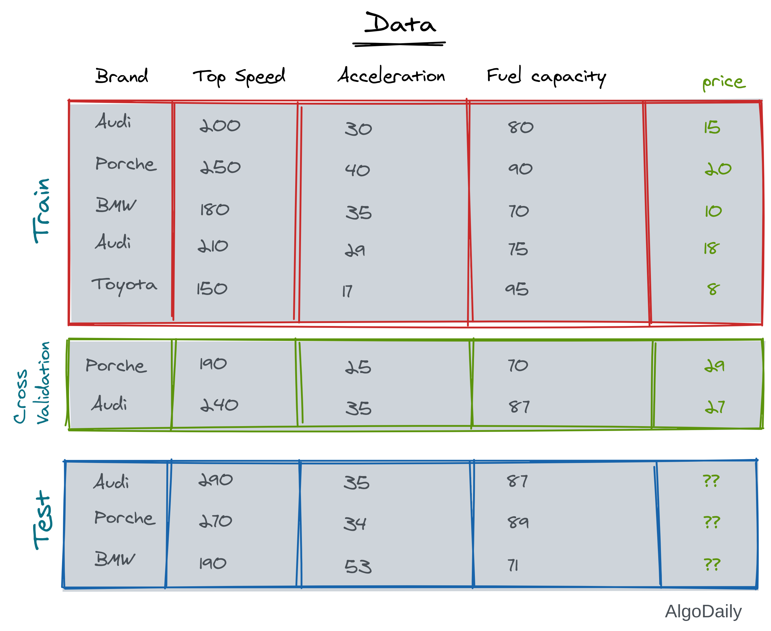
1. Training Data: This is the data that we know everything about. We know what should be the output of this data. So we can calculate the loss of our model from this data. We can also calculate the accuracy of the model from this training data. This is the data that is used in the training loop of an ML algorithm. In the example above, all the features along with the prices are the training data.

2. Test Data: This is the data that we need to understand using our ML algorithms. We need to predict the result of unknown data with our model. Suppose you learned a model from the given training data of vehicles. Now if you have the feature lists of a set of cars, and you do not know their price, that will be your test data.

So if you train on the whole training data, you will not have any solid way to test the accuracy of your model. Maybe your model will work on seen data but will break on unseen data. You won’t be able to get the accuracy from your test data because you do not know the prices of vehicles of the test data. To solve this, the training data is again divided into two parts.

1. Actual Train Data: This data is the actual training data that will be used in the training loop. In most cases, this is 80% or 75% of the whole train data.

2. Cross-Validation Data: This is kept separate from the actual training data and is not used in the training loop. So after training, this cross-validation data is unseen to the model. So we can cross validate our model on both seen and unseen data from the train data. Most of the time, this data is 20% or 25% of the training data.

Dataset attributes have a classification according to their usage:

1. Feature: These are the attributes or columns that the machine learning model will analyze and learn. In the vehicle dataset, all the columns except price are features.

2. Label: These are the attributes or columns that the machine learning model will try to predict. This label will be used to calculate loss and accuracy. In the vehicle dataset, the column “price” is the label.

To illustrate the whole scenario with the vehicle dataset example, look at the image above. The prices in green are the label of the data, and the rest of the columns are features. We will understand more about different types of features like numeric, categorical features, etc soon.

Different classes of Machine Learning

There are many kinds of machine learning algorithms depending on the objective and provided data. We will discuss some of them below:

Supervised Learning and Unsupervised Learning

These classes of learning are the most popular among all. If the provided data has a label on it, then it is supervised learning. If the process or algorithm does not need any label, then it is unsupervised learning.

The above model for the vehicle dataset is supervised learning if you want to predict the price or any feature from the rest of the attributes. The same data can be used for unsupervised learning if you want to cluster similar vehicles or detect outlier vehicles.

Usually, unsupervised learning is a little harder than supervised learning. Because it is difficult to determine the loss or goodness of a model as there is no label to compare with. For clustering a dataset, you can use the distance between the mean of two clusters or inverse of distance among points in similar clusters as goodness of the model. We will first encounter many supervised learning methods. Later on in this series, we will go through data clustering, outlier detection, data augmentation, synthesis, and many other unsupervised learning applications.

Instance-based Learning and Model-based Learning

Machine learning can be divided into two categories based on the learning process and weights management.

Think of the example ML program you implemented at the beginning of this lesson. Is the weight guess saved somewhere for future use? Can the model work better for a later case when you guess a different number? No. This is what instance-based learning is. In instance-based learning, the algorithm works for only the current instance of the data. It is highly dependent on the data and does not work later if you do not provide data.

On the other hand, some ML algorithms can save their weights for later use. These kinds of algorithms can relearn and improve themselves if more data is provided. When doing prediction, it does not depend on the data. All the deep learning algorithms are model-based learning processes.

Instance-based learning algorithms are usually faster than model-based learning. For example, the Bayesian network model or KNN clustering algorithm is always faster than a deep learning algorithm when learning.

Offline/Batch Learning and Online Learning

Depending on the data again, ML algorithms can be divided into two kinds. Machine learning algorithms can learn while the data is given live, or learn after getting the complete dataset provided at once.

In the above number guessing program, the data is given to the computer one by one. The data looked like the following at each step:

1
2
3
4
5
6

Step 1: 99 is bigger than guess
Step 2: 89 is bigger than guess
Step 3: 79 is bigger than guess
Step 4: 69 is bigger than guess
Step 5: 59 is bigger than guess
...

This type of learning algorithm is known as the Online learning process. The data is given live while the training loop is running.

On the other hand, if you try to do a dog-cat classification, many images of dogs and cats are given to the learning model at once. The model runs for several epochs for all the images and then gets ready to predict a test image. This kind of learning is Offline/Batch learning. Because we are providing a batch of dataset at once.

Conclusion

This lesson is very important to understand for your Machine learning career. This is the fundamental of machine learning. We will go through some core mathematics behind ML in the next lesson. I would recommend you go through the algorithm multiple times, print different variables in the training loop, and understand the whole process.