Deep Learning and Computer Vision

Introduction

In the previous lesson, you were introduced to one of the most popular frameworks for Deep Learning, TensorFlow. In this lesson, we will use TensorFlow to create some popular deep neural networks. In the meantime, you will also learn which deep learning technology should be used with what kind of data, and how you can customize a deep neural network to your needs. So let us get started.

Neural Network for Image Data

First, we will start with Image datasets. There is a whole different field for images, videos, and other visual data (LIDAR, X-Ray, Depth Camera, etc.) called Computer Vision. One of the most compelling types of AI is computer vision which you’ve almost surely experienced in any number of ways without even knowing. Some of the examples are:

• You have used face filters in Snapchat, Facebook Messenger, YouCam Perfect, etc. apps, right?
• For security purposes, sometimes an object from a video or image is blurred/removed/pixelated. With CV, you can do that efficiently.
• You might have used google translate’s image to text feature. It takes an image and reads the text within it.
• There are many examples of image classification. For example, many machines use image processing to classify different coins and notes.

All of the above applications of Computer Vision are done using Deep Learning. That is why, nowadays, you cannot imagine Image processing without deep learning.

To get started with deep learning, we need to have a look at how images are stored in a computer.

Structure of an Image

There are many formats of images (png, jpg, BMP, tiff, etc.). But when an image is loaded for processing in the memory, trivially it is loaded as a 3-dimensional tensor. So images are tensor objects whose dimension is always 3.

Among these three dimensions, the first two dimensions are for the height and width of the image. These only two dimensions together form a matrix that represents a channel of an image. Mostly, this is a color channel. The third dimension represents the number of channels of the image. For example, if the shape of an image is (500, 600, 3), that means the image is 500 pixels high, 600 pixels wide, and has 3 color channels.

Depending on the number and order of color channels, images can be in different color formats. Some examples of these formats are given below:

1. RGB: This is the simplest and most popular format. Images have 3 color channels, represents Red, Green, and Blue (RGB). Keep the order in mind because in RGB, always the first channel is for the color Red, the second is for Green and the third is for Blue.
2. RGBA: If you add an alpha channel to the RGB image, then you get RGBA images. These images have opacity. PNG image formats are compatible with RGBA image format as they also have this opacity channel.
3. BGR: Blue, Green, and Red channels in the image. This is the same as RGB but the order of the channel is different. Although this format is not that popular, for some reason the most popular computer vision library OpenCV used this format as default.
4. Grayscale: There is only one channel of the image. You can represent it in both (h,w,1) or just (h,w) format.

All the above formats consist of pixels/color values which can be represented again in two ways.

In computer vision, there are also other data formats. For example, there is a voxel (Volumetric Pixel). This format is a four-dimensional tensor of share $(h,w,d,c)$, where they represent the height, width, depth, and channel respectively. There are also Point Cloud representations for a LIDAR dataset. As we are covering the basics, we will only stick to the formats mentioned above.

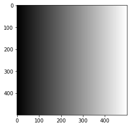
Let us define an image by ourselves. In the below example, we will create a gradient grayscale image and display it.

 1
 2
 3
 4
 5
 6
 7
 8
 9
10
11
12

import numpy as np
import matplotlib.pyplot as plt

def get_gradient_2d(start, stop, width, height, is_horizontal):
    if is_horizontal:
        return np.tile(np.linspace(start, stop, width), (height, 1))
    else:
        return np.tile(np.linspace(start, stop, height), (width, 1)).T

img = get_gradient_2d(0, 255, 500, 500, True) # shape = (500, 500)

plt.imshow(img, cmap="gray")

And here is the result:

OpenCV

Image processing and Computer Vision are vast fields of study in both academics and industry. It is simply infeasible for anyone to use primitive libraries like NumPy for image manipulation. For this, many specialized image processing libraries are created. Among them, OpenCV is by far the most popular Image processing library. It is fast, written in C++, ported to many programming languages like Java, JS, Python, C#, etc. It can not only processing images but also read different image formats, convert between different formats, read/write to different kinds of source and sink devices like webcam, video file, image file, etc. The world of image processing and computer vision is just incomplete without this amazing library.

As I said earlier, the default image format for OpenCV is BGR. So to work with all other libraries, you need to convert the image to RGB or RGBA first. Let us see an example where we read an image and display it with matplotlib. You can download the famous image processing sample picture of Leena from here.

1
2
3
4
5

import cv2
img = cv2.imread('leena.png')
img = cv2.cvtColor(img, cv2.COLOR_RGB2BGR)
print(img.shape)
plt.imshow(img)

If you run the code, you will see that the image is of shape (463,453,3). The result will look something like this.

Did you notice the integer flag named cv2.COLOR_RGB2BGR while converting an image? Get used to it, OpenCV uses hundreds of integer flags like that. You need to use those flags as parameters of its methods.

Image Preprocessing

You already know that, in machine learning, the first step after loading data is preprocessing. In python, preprocessing images is mostly done with NumPy and OpenCV. In this lesson, we will focus on the preprocessing parts that are needed for feeding it into a neural network. Below are the four things you have to do before feeding images into your network.

1. Resizing: All neural networks have to take in the same tensor shapes. For this, you need to find the right size for all your images and then resize all images into that size. You can use the cv2.resize(img, shape) method for resizing. For image resizing, you also need to know about different interpolation techniques. The most common one used is cv2.INTER_NEAREST which can be passed to the function while resizing.
2. Intensity Scaling: Each pixel value of images is in a range from 0 to 255 most of the time. But to get the best result, it is proved that the range of pixel values should be between 0 and 1, or -1 and 1. You can use the skimage.exposure.rescale_intensity(img) method from scikit-image module to rescale images to any range. The background is the same as rescaling any attribute in a dataset which we did previously.
3. Quantizing: In your given images are not photos of scenarios with a wide range of colors, quantizing your images and just inputting only 5-10 color values instead of 255 will drastically improve your model’s prediction speed. Besides, for certain types of images (region of interest of object detection for example) this method will also increase the accuracy of your model. You need to do this manually using NumPy.
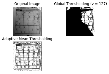
4. Thresholding: If you only need a certain color or range of color, then you can apply a threshold to that range of color in your image. There are many kinds of thresholds’ that you can do. First, let us look at some simple threshold methods OpenCV offers us. Each threshold method is briefly described above the method in comments. We will work with the gradient image we created with NumPy.

 1
 2
 3
 4
 5
 6
 7
 8
 9
10
11
12
13
14
15
16
17
18

img = cv.imread('gradient.png',0)
# All pixels above 127 will be 1, others will be 0
ret,thresh1 = cv.threshold(img,127,255,cv.THRESH_BINARY)
# All pixels above 127 will be 0, others will be 1
ret,thresh2 = cv.threshold(img,127,255,cv.THRESH_BINARY_INV)
# Make all pixels greater that the value 127 to the value 255
ret,thresh3 = cv.threshold(img,127,255,cv.THRESH_TRUNC)
# Make all pixels greater that the value 127 to the value 0
ret,thresh4 = cv.threshold(img,127,255,cv.THRESH_TOZERO)
# Make all pixels less that the value 127 to the value 0
ret,thresh5 = cv.threshold(img,127,255,cv.THRESH_TOZERO_INV)
titles = ['Original Image','BINARY','BINARY_INV','TRUNC','TOZERO','TOZERO_INV']
images = [img, thresh1, thresh2, thresh3, thresh4, thresh5]
for i in range(6):
    plt.subplot(2,3,i+1),plt.imshow(images[i],'gray',vmin=0,vmax=255)
    plt.title(titles[i])
    plt.xticks([]),plt.yticks([])
plt.show()

The result of the code is below.

These threshold algorithms have a fixed function, that is applied to all the pixels, regardless of the value of that pixel or its neighborhood. These kinds of threshold algorithms are call global threshold algorithms. There are also local/adaptive threshold algorithms. These adaptive threshold algorithms take a neighborhood into consideration and then apply threshold to some pixels. We will discuss only one threshold algorithms, adaptive mean threshold. This algorithm takes an kernel sized neighborhood and takes the mean of that kernel as the thresholding value. Then it applies the thresholding on that region. OpenCV has cv2.adaptiveThreshold function for this. Let us see what it does in realtime:

 1
 2
 3
 4
 5
 6
 7
 8
 9
10
11
12
13

img = cv2.imread('sudoku.jpg',0)
img = cv2.medianBlur(img,5)
ret,th1 = cv2.threshold(img,127,255,cv2.THRESH_BINARY)
th2 = cv2.adaptiveThreshold(img,255,cv2.ADAPTIVE_THRESH_MEAN_C,\
            cv2.THRESH_BINARY,11,2)
titles = ['Original Image', 'Global Thresholding (v = 127)',
            'Adaptive Mean Thresholding']
images = [img, th1, th2]
for i in range(3):
    plt.subplot(2,2,i+1),plt.imshow(images[i],'gray')
    plt.title(titles[i])
    plt.xticks([]),plt.yticks([])
plt.show()

Finally, we will discuss the last and most popular threshold algorithm. You do not have to select a threshold value (like we did 127 for all the above examples). The algorithm will select the optimal threshold value which will divide the whole image into the best binary regions. It is OTSU’s binary threshold algorithm. Before understanding this algorithm, you need to learn about the histogram of images.

Histogram of Images

Each pixel of images has a range of values. It can be a discrete/quantized number of values: for example integer values from 0 to 255. They can also be continuous values ranging from 0.0 to 1.0. Either way, you need to plot a graph of the distribution of pixel values of the image using a 2D line plot. The X-axis will represent the range of the values. So it can be in between 0-255 or 0-1. The Y-axis represents the number of pixels for the corresponding pixel value in the X-axis. For example, if an image has a total of 400 pixels whose values are 55, then the Y value of the plot at $X=55$ is $400$. So the maximum value of Y-Axis would be $hw$ where $h$ is height and $w$ is the width of the image.

Matplotlib provides us utility function to get the histogram of an image. Let’s see how the histogram of a binary image looks like.

1
2
3

img = cv2.imread('ex.jpg',0)
plt.hist(img.ravel(),256,[0,256])
plt.show()

As you can see, most of the pixels’ color values are around 100.

OTSU’s threshold algorithm uses this histogram information to calculate the optimal value to threshold an image. Otsu’s algorithm tries to find a threshold value (t) that minimizes the weighted within-class variance. We will not get into the mathematical details of this algorithm (it is quite interesting to look at though). OpenCV provides cv2.threshold(img,0,255,cv2.THRESH_BINARY+cv2.THRESH_OTSU) function that can be used for this. There are many online documentations to look for on the internet. Sometimes, applying a blurring (e.g. Gaussian Filter) will make the result of the threshold algorithm much better.

For preprocessing, you can also apply histogram equalization to make the color distribution of all the images very similar. It is appropriate in the case of digit classification or character recognition. I will cover all these image processing techniques in a later lesson.

Image Classification with Deep Learning

Now we are at the heart of today’s lesson. We will use 2 types of neural networks on the popular Fashion MNIST dataset to classify 10 different fashion images. In the previous lesson, I presented you with how to easily create a neural network using TensorFlow within just 10 lines of code. We use that same code to create a digit classifier in this lesson.

Although I will only show you an image classification example, there are many other principle tasks for deep learning. The most common types are:

A. For single Object

1. Image classification: Is this object in the photo?
2. Image classification: What object (among some predefined) is in the photo?
3. Object localization: Where is this object located in the image?
4. Object segmentation: Just select those pixels which are part of an object in the image.

B. For multiple objects in the same image:

1. Object detection: Where each object is located in a single image?
2. Instance Segmentation: Classify all pixels of an image to mark it as a part of some object (or background).

A famous image for understanding these types is shown by Mike Tamir.

Linear Neural Network

Linear neural networks are built with neurons where each neuron is responsible to select/determine if a feature in that value is present. When you add a lot of neurons to a single layer, it tries to detect specific features in the whole dataset that will help you to achieve the final goals. The first layer of the network is only able to detect simple features in the data. Later layers take in the detected features from the previous layers and detect more complex features among them.

For images, each neuron will take in all the pixels at once, and try to predict a number. That prediction number can mean anything (mostly unrecognizable by humans). Next, that value will be again propagated to all the neurons on the next layer. For classification, the output layer will have only 10 neurons. Each neuron will be responsible to predict a value that tells us how much is it likely, that the image is $n \n {0…9}$.

Images are a tensor of 3 dimensions. MNIST images are grayscale images, so they are actually of 2 dimensions (So the whole dataset is of shape (8000, 28, 28)). But Linear neural networks only take a dataset with a linear feature set. Each feature can contain only 1 value for sample data. So we need to convert each of our images into a linear example. We can do this pretty easily by flattening each image using the NumPy flatten method. But then we need to loop through all the images and call the method on each of them. Instead, we can just use the np.reshape method to reshape the whole dataset into the desired shape.

Before that, lets import all the libraries we need for this:

 1
 2
 3
 4
 5
 6
 7
 8
 9
10
11
12
13
14
15

# Basic
import pandas as pd
import numpy as np

# for visualization
import matplotlib.pyplot as plt

# Creating the model
import tensorflow as tf
from tensorflow.keras.models import Sequential
from tensorflow.keras import layers
from tensorflow.keras.wrappers.scikit_learn import KerasClassifier

# To Evaluate the models
from sklearn.model_selection import cross_val_score, cross_validate

Next, we load the dataset into memory. We will use TensorFlow’s dataset submodule to load the dataset. It will download the dataset from the internet and return it to a python variable.

1
2

mnist = keras.datasets.fashion_mnist
(X_train, y_train), (X_test, y_test) = mnist.load_data()

After loading the dataset, we will reshape the dataset into our desired linear shape. We might not know the number of samples for the data, so we can use the shape of the NumPy dataset to get the number of examples in both of our training and testing sets. After reshaping the dataset, we will do a very simple preprocessing. The range of color of the pixel is 0-255. We will divide it by 255 so that we can get a range from 0-1. This is necessary for most deep neural networks or there might be exploding gradient problem.

 1
 2
 3
 4
 5
 6
 7
 8
 9
10

# Reshape each iamges from 2D to 1D array.
# So the whole dataset is now 2D
X_train = X_train.reshape(X_train.shape[0], 784)
X_test = X_test.reshape(X_test.shape[0], 784)

y_train = to_categorical(y_train)
y_test = to_categorical(y_test)

X_train = X_train / 255.0
X_test = X_test / 255.0

Now that our data is ready and preprocessed, let’s have a peek at some of the images we are dealing with. Data visualization is very important for any model development as it gives you insights into different approaches you can take with your data and model. In this dataset, here each class label [0..9] represents a cloth/shoe in the dataset.

1
2
3
4
5
6
7

fig, axes = plt.subplots(nrows=2, ncols=5,figsize=(15,5))          
ax = axes.ravel()
for i in range(10):
    ax[i].imshow(X_train[i].reshape(28,28), cmap="gray")
    ax[i].title.set_text('Class: ' + str(np.argmax(y_train, axis=1)[i]))              
plt.subplots_adjust(hspace=0.5)                                    
plt.show()

Now we will build our Artificial Neural Network (ANN). The model will consist of only 1 hidden layer (because the dataset is very simple). We will use uniform weight initialization, categorical cross-entropy for loss, and Adam optimizer.

 1
 2
 3
 4
 5
 6
 7
 8
 9
10
11
12
13
14

# Create a model (we will use Sequential API)
model = Sequential()
# Input layer
model.add(layers.InputLayer(X_train.shape[1]))
# Hidden layers
model.add(layers.Dense(128, kernel_initializer='uniform', activation='relu'))
# Output layer
model.add(layers.Dense(10, kernel_initializer='uniform', activation='softmax'))

# Add accuracy as metric and categorial crossentropy as loss, optimizer adam
model.compile(optimizer='adam', loss='categorical_crossentropy', metrics=['accuracy'])


model.summary()

The model summary output is:

 1
 2
 3
 4
 5
 6
 7
 8
 9
10
11

Model: "sequential"
_________________________________________________________________
Layer (type)                 Output Shape              Param #   
=================================================================
dense (Dense)                (None, 128)               100480    
_________________________________________________________________
dense_1 (Dense)              (None, 10)                1290      
=================================================================
Total params: 101,770
Trainable params: 101,770
Non-trainable params: 0

Finally, we train the model with the X_train and label y_train.

1

model.fit(X_train, y_train, epochs=10)

We will see the training progress at each epoch. After training the model, we can evaluate the model on the test set.

1

model.evaluate(X_test, y_test)

The result is 87% accuracy. Keep in mind that if you tune the model, preprocess the data properly, it is possible to get 90+ accuracy with just a linear neural network. And 99.99% accuracy is possible if you train these image datasets into a well-developed Convolutional Neural Network.

Convolutional Neural Network

Convolution Operation

Convolutional Neural Network is the most efficient neural network developed for images until now. There are a lot of variations of CNN out there. In this lesson, I will try my best to make CNN as much clarity as possible. The first thing to understand for CNN is how convolution operation works.

In purely mathematical terms, convolution is a function derived from two given functions by integration which expresses how the shape of one is modified by the other. That can sound baffling as it is, but to make matters worse, we can take a look at the convolution formula:

$$(f*g)(t) = \int_{-\infty}^{\infty} f(\tau)g(t-\tau) d\tau$$

So let us not think about the mathematical background, and see a practical example.

The convolution operation is done on an image (for this context) with a kernel. Most of the time, the kernel is much smaller in size than the image. Suppose the image is a (5x5) matrix, and the kernel is a (3x3) matrix.

 1
 2
 3
 4
 5
 6
 7
 8
 9
10
11
12
13

A = [
  [1,2,3,4,5],
  [5,4,3,2,1],
  [6,7,8,9,8],
  [3,4,5,6,7],
  [5,4,3,2,1],
]

k = [
  [1,2,3],
  [3,2,1],
  [4,5,6],
]

The convolution between these two will result in an image of shape (4,4). The kernel will start from the top left corner of the image (where it can fit inside the image). Then it will element-wise multiply and sum up all to get a single value.

1
2
3
4
5
6
7

[
  [1x1 + 2x2 + 3x3] +
  [5x3 + 4x2 + 3x1] + 
  [6x4 + 7x5 + 8x6] + 
]

= 147

Then the kernel will again shift to the right by 1 and again do the same operation to the submatrix and the kernel.

1
2
3
4
5
6
7

[
  [2x1 + 3x2 + 4x3] +
  [4x3 + 3x2 + 2x1] + 
  [7x4 + 8x5 + 9x6] + 
]

= 162

This process will continue until a place where the kernel does no more fit in the image. Then the kernel will start over from the left of the image, going down 1 pixel. So after the first row, the first result of the second row will look like this:

1
2
3
4
5
6
7

[
  [5x1 + 4x2 + 3x3] +
  [6x3 + 7x2 + 8x1] + 
  [3x4 + 4x5 + 5x6] + 
]

= 124

This will continue until the end, and the resulting image will be the summing value put in the center of the kernel while the multiplication operation was being done. This will result in a (4x4) matrix. As you always have to select the center location of the kernel to place a pixel value, kernel shape cannot be even size.

1
2
3
4
5

A * k = [
  [147, 162, 165],
  [124, 139, 152],
  [124, 121, 112],
]

Using OpenCV, you can apply the convolution operation using filter2D(img, -1, kernel) function. But OpenCV tries to keep the output the same size as input. To keep this same shape, it first adds a border to the image so that after applying the convolution, the result is of the same shape as the input image. There are many cv2.BOARDER* flags that you can use to specify different ways to pad the image. We will just ignore them for now and only take the image as output:

 1
 2
 3
 4
 5
 6
 7
 8
 9
10
11
12
13
14
15

A = np.array([
  [1,2,3,4,5],
  [5,4,3,2,1],
  [6,7,8,9,8],
  [3,4,5,6,7],
  [5,4,3,2,1],
], dtype='uint8')

k = np.array([
  [1,2,3],
  [3,2,1],
  [4,5,6],
], dtype='uint8')

cv2.filter2D(A, -1, kernel=k)[1:-1, 1:-1]

The resulting image is:

1
2
3

array([[147, 162, 165],
       [124, 139, 152],
       [124, 121, 112]], dtype=uint8)

CNN Layer

CNN is a neural network based on 2D convolution operation. The values in the kernel are considered as weights. You can select a kernel initialization method (uniform, he_uniform, etc.) and the size of the kernel. At each training iteration, the weights of the kernels will be updated with the loss and gradient in the backpropagation step.

In TensorFlow, the code will not be different from that of the linear neural network. The Dense layers of the model definition will only be replaced with Conv2D layers. Let’s see the whole code at once:

 1
 2
 3
 4
 5
 6
 7
 8
 9
10
11
12
13
14
15
16
17
18
19
20
21
22
23
24
25
26
27
28
29
30
31
32
33
34
35
36
37
38
39
40
41
42
43
44

# Basic
import pandas as pd
import numpy as np
import tensorflow as tf

# for visualization
import matplotlib.pyplot as plt

# For preprocessing the data
from tensorflow.keras.utils import to_categorical

# Creating the model
from tensorflow.keras.models import Sequential
from tensorflow.keras import layers


mnist = tf.keras.datasets.fashion_mnist
(X_train, y_train), (X_test, y_test) = mnist.load_data()

# We do not need to reshape the images into a linear datashape. 
# CNN takes an image as input with different number of channels you define
# These are grayscale images, so the number of channels is one
X_train = X_train.reshape(X_train.shape[0], 28,28,1)
X_test = X_test.reshape(X_test.shape[0], 28,28,1)

y_train = to_categorical(y_train)
y_test = to_categorical(y_test)

X_train = X_train / 255.0
X_test = X_test / 255.0

model = Sequential()
model.add(layers.InputLayer((28,28,1)))
model.add(layers.Conv2D(32, (3, 3), activation='relu', kernel_initializer='uniform'))
model.add(layers.MaxPooling2D((2, 2)))
model.add(layers.Flatten())
model.add(layers.Dense(100, activation='relu', kernel_initializer='uniform'))
model.add(layers.Dense(10, activation='softmax'))
# compile model
opt = tf.keras.optimizers.SGD(learning_rate=0.01, momentum=0.9)
model.compile(optimizer='adam', loss='categorical_crossentropy', metrics=['accuracy'])

model.fit(X_train, y_train, epochs=10)
model.evaluate(X_test, y_test)

If you have a GPU (and you properly installed TensorFlow, CUDA, and everything else to use GPU following our previous tutorial), then this will take less than a minute. But if you are running TensorFlow on CPU, you might want to grab a coffee because it will take about 4-5 minutes.

The evaluation result is 90%. This is higher than a linear neural network. All the other hyperparameters other than the model architecture are the same. So you can see that for image operations, CNN is better than trivial ANN.

More Neural Networks: How to explore them?

People worry that computers will get too smart and take over the world, but the real problem is that they’re too stupid and they’ve already taken over the world

• Pedro Domingos

Developing a machine learning model is just a part of Art. There are no hard rules on how to develop the perfect machine learning model. You just have to be experienced enough to have a good feeling that “these” kinds of models should work well on these kinds of data. One can create a very wide neural network for a task, and another person can create a very deep and narrow neural network. None of them are guaranteed to work perfectly and any of them can fail training properly.

So you need a lot of experience to create good neural network architectures. You will need to see and run models developed by other experts out there. There are many websites where you can find different state-of-the-art neural network models for different kinds of data. I am listing below some of the most popular ones you want to look at.

1. ModelZoo.com: https://modelzoo.co/
2. ONNX Model Zoo: https://github.com/onnx/models
3. Keras Applications: https://keras.io/api/applications/
4. IBM exchange model repository: https://developer.ibm.com/exchanges/models/
5. Computer Vision Model Library: https://models.roboflow.com/

It seems that all the major deep learning framework owners have their deep learning model repositories.

1. TensorFlow: https://github.com/tensorflow/models
2. PyTorch: https://github.com/Cadene/pretrained-models.pytorch
3. caffe: https://github.com/BVLC/caffe/wiki/Model-Zoo
4. caffe2: https://github.com/caffe2/caffe2/wiki/Model-Zoo
5. Lasagne: https://github.com/Lasagne/Recipes

I think these will be enough, for now, to try some machine learning models by yourself. Many of these are pre-trained models, so you only need to use them for prediction. But you may also want to train a model with a dataset. Let us discuss where to find a dataset that you can use in your own software.

Dataset: Where to find them?

The best place to find a dataset is Kaggle-Datasets. Besides kaggle, you can look at the following websites to search for a dataset:

1. UCI Machine Learning Repository: https://archive.ics.uci.edu/ml/
2. Awesome Public Dataset: https://github.com/awesomedata/awesome-public-datasets
3. Microsoft Research Open Data: https://msropendata.com/
4. Amazon Open Data Registry: https://registry.opendata.aws/
5. Visual Data Discovery: https://www.visualdata.io/discovery

If you do not want to browse these repositories, you can use Google to do it for that. But not the google.com. It is Google Dataset Search Engine

There are also government-sponsored public datasets for many countries. Some of the popular ones are:

1. US Gov Data: https://www.data.gov/
2. Indian Government Dataset Repository: https://data.gov.in/
3. European Government Datasets: https://data.europa.eu/euodp/data/dataset
4. New Zealand’s Government Dataset: https://catalogue.data.govt.nz/dataset
5. Northern Ireland Public Dataset: https://www.opendatani.gov.uk/

Tell us in the discussion section if your country has a dataset repository.

Conclusion

This is the end of the deep learning on image dataset lesson. In this lesson, I tried to mention all you need to know about computer vision and deep learning. I did not go thoroughly into any topic because most of the libraries are open source and you can get to their official tutorials which will be better than any other place. This will also help you to learn to read official documentation.