Hands-on first Machine Learning Algorithm from Scratch

Introduction

Previously, we have created a program, that behaves almost like a machine learning algorithm. But in this section, we will officially create our first machine learning program. We are going to implement linear regression.

Objective

Our objective is to predict house prices based on several features of a house. As there is more than one feature for this dataset, the task is a multivariate linear regression.

Go ahead and grab the Kaggle competition dataset from the website. We will only need the train.csv file from the dataset.

Reading the data

Let us first start with the data acquisition and preprocessing. We grab the data just like we did in the last lesson.

1
2
3
4
5
6

import pandas as np
import numpy as np

#%%
df = pd.read_csv('train.csv')
df.head()

Data shuffling

In many cases of data acquisition, the data seems to be written to a CSV file in an orderly manner. For example, the data can be there in order of SalesPrice or any other feature. But in this house price prediction case, there is no actual meaning to the order of the houses in the CSV file. We do not want our ML algorithm to pick this order and learn something from it. So it is always a good idea to shuffle the data first if there is no meaning in the ordering of the data.

Shuffling can be done in many ways with many libraries. As we only have introduced pandas and NumPy, we will shuffle the CSV directly through pandas sample method. Later you will know that it is even easier to shuffle with just shuffle(data) using scikit-learn.

1

df = df.sample(frac=1).reset_index(drop=True)

We are sampling the data (all the data because we put fraction=1) which is the same as shuffling. When sampled, pandas try to keep the index of the shuffled data the same as the original one. This will create a problem if we want to access data using Loc. We can reset the index with the reset_index method.

Preparing features and Labels

After shuffling the data, we preprocess the data to directly feed to an algorithm pipeline. The only numerical features we are going to use are OverallQual, GrLivArea, and GarageCars. The label will be SalesPrice. So we will take only these 3 columns into the input data X and 1 column to label data y.

1
2

x = df[['OverallQual', 'GrLivArea', 'GarageCars']].to_numpy()
y = df['SalePrice'].to_numpy()

Input feature normalization

You can notice that the input feature x has different ranges for different columns. We will later use a gradient descent algorithm for optimizing the loss. You will start to understand in a moment, but the gradient descent algorithm works badly when different data are in different ranges. We can solve this by normalization.

The equation of normalization is as follow:

1

X_new = (X - mean(X_old)) / standard_deviation(X_old) ; X is a column representing a feature of all samples

We will also add a column of 1s to the feature set. We will explain the reason in a bit when discussing the prediction process.

1
2

x = (x - x.mean(axis=0)) / x.std(axis=0)
x = np.c_[np.ones(x.shape[0]), x]

We could also do min-max feature scaling if we wanted. The result will be almost similar.

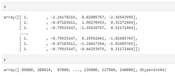
After processing, the data will look something like this:

Splitting the data to Train and Test

As the data is already shuffled, we can just take the first 90% of the data for training, and 10% of the data for validation. This can be done with NumPy’s slicing operation.

1
2
3
4
5
6
7

X_train = x[:int(len(x)*0.9)]
X_test = x[int(len(x)*0.9):]

y_train = y[:int(len(y)*0.9)]
y_test = y[int(len(y)*0.9):]

X_train.shape, y_train.shape, X_test.shape, y_test.shape

Gradient Descent Algorithm

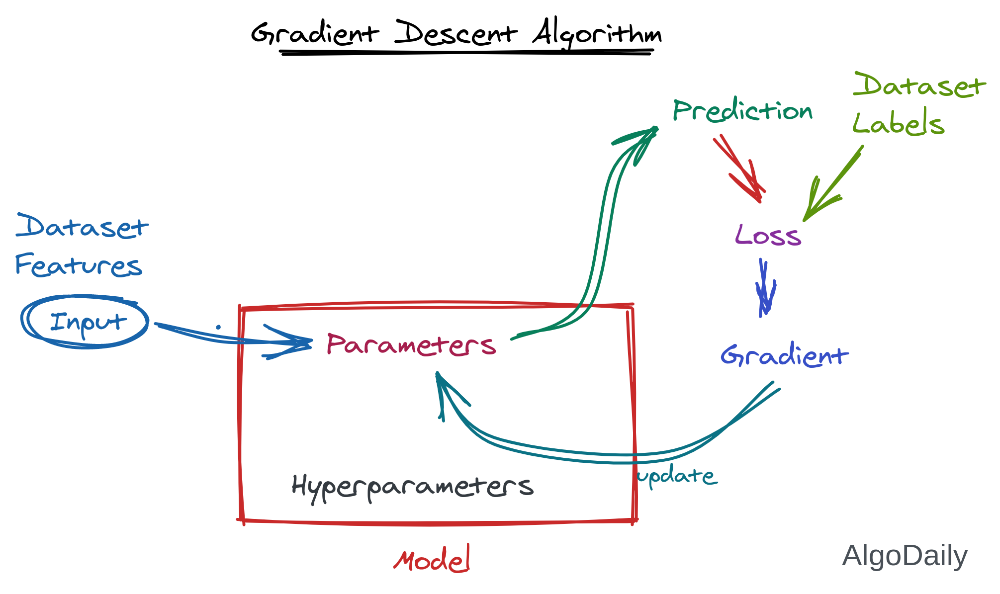
Nowadays, gradient descent algorithms remain pretty much the same for all the algorithms from stochastic linear regression, to advanced deep learning. This algorithm needs to have a loss function (loss_i), and a learning rate parameter. All this algorithm does is subtract the gradient of loss of all samples from the original weight at each learning iteration. The actual derivation of the algorithm requires a good knowledge of calculus and is left for self-learning. The updating speed of the weight can be controlled using the learning rate (alpha) parameter (just like the decrement_jump in the guessing game).

Let us see the equation to update weight directly from Wikipedia:

Here, the parameter that needs to be updated is a. At every learning iteration, it will be updated by the gradient of loss. $x_n$ is the $n$th sample and $F(x_n)$ is the loss of that sample. The $\Delta F(x_n)$ defines the gradient of loss. This is actually the differentiation of loss with respect to the input. Without burning our brains too much, the calculated result of the derivative of loss (the gradient) is half of the dot product of input matrices transpose with the loss.

The simplified equation goes something like this.

$$
weight_{n+1} = weight_n - lr * 0.5 * X^T.loss
$$

This updating process will happen a fixed number of times, which is known as the number of epochs. We can keep track of the losses during the training loop in an array cost_history.

1
2
3
4
5
6
7
8

def gradient_descent(X, y, w, lr, epochs):
    cost_history = np.zeros(epochs)
    for i in range(epochs):
        errors = predict(X, w) - y
        grad = (1 / len(X)) * X.T.dot(errors) # mse can also be calculated with matrix dot product
        w = w - lr * grad
        cost_history[i] = loss(X, y, w)
    return w, cost_history

Prediction and Loss Function

Let us think of the loss function as a subtraction between the prediction and label. This is for only one sample of data. But for a batch of sample data, we need to normalize the loss. We can sum all the individual losses and divide them by the number of samples. It is not always necessary, but for some derivation explanatory reasons, the loss is further divided by 2.

1
2
3
4

def loss(X, y, w):
    errors = predict(X, w) - y
    pred_loss = 1/(2 * len(X)) * errors.T.dot(errors)
    return pred_loss

The prediction or output will be the multiplication of the weights and the input feature set. This came from the equation $y = w * x + b$. Here, $x$ is the input features, and $w$ is the weights that gradient descent will learn. Remember that we added a column of 1s while preprocessing the data? That $1$ is called bias, $b$ in the equation. We can implement this on python pretty easily because we already prepared our data to be compatible with bias.

1
2

def predict(X, w):
    return X.dot(w)

The Training Loop

All the functions are now defined properly. The starting of the program will be the initialization of all the parameters. There are two types of parameters in ML algorithms.

1. Training Parameters: These are the parameters that are updated in the training loop. These are also simply called parameters. This can be only a single floating value or a tensor of size more than gigabytes.

2. Hyperparameter: These are the parameters of the parameter updating process. These are set by us before running the algorithm. Examples are learning rate, number of epochs, parameter initialization distribution, etc.

1
2
3
4
5
6

# Initialize parameters
w = np.zeros(4)

# Initialize hyperparameter
epochs = 800000;
lr = 0.15;

Then we call the gradient descent function and the model will be trained.

1
2
3

w, cost_history = gradient_descent(x, y, w, lr, epochs)
print('Initial loss =', cost_history[:5].mean())
print('Loss after training =', cost_history[-5 :].mean())

We can clearly see that the loss is decreased. So our model has learned something meaningful from the feature set.

Conclusion

In this lesson, you have officially created the first well-established machine learning algorithm. You became familiar with the math behind the most popular machine learning algorithms, gradient descent. I will recommend you to go through the whole algorithm, print variables at different lines in the python code to understand how it is actually working. In most of the applications in machine learning, you won’t be using this type of code that much; thanks to many modern python modules that implement this algorithm for us. Finally, as an exercise, you can grab any other dataset online and try to preprocess and apply this algorithm to predict something new. Don’t forget to share your experience and problems with us about your new implementation in the discussion section.