
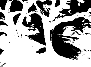
Rotate each of the 3D pointclouds horizontally 90° to see the other view.
The next one is a little complicated with real binary images. The reconstruction is not great, but we can see similarity in the image and perspective easily.

Disclaimer
This work is done as a side project of MPSE MDS. Without any duplications, I would suggest to go through that post first before this one.
Presentations
Introduction
Following the original MPSE paper, I tried to implement the algorithm by myself. But, initially I could not get any result with my own implementation, maybe then I did not understood how SGD works with the given stress function. It seems that Stochastic Gradient Descent was not able to minimize the stress function at all (in my implementation).
\begin{equation}
\underset{x \in !R ^{p \times n} }{\text{minimize}} \sum\limits_{k=1}^3 \sum\limits_{i > j} (D_{ij}^k - || P^k(x_i) - P^k(x_j) ||)^2 \
\label{eq:stressmin}
\end{equation}
Later, I started to think about how this can be done in many other ways. I found a new approach which I named mpse-gan.
MPSE-GAN
Primarily, what 3D reconstruction with mpse is doing is generating a set of 3D points that look like a given set of points from the real world from a 2D perspective view. This is exactly what Generative Adversarial Networks can be very good at.
We tried a discriminating neural network with a slightly modified loss function of yours to predict whether a 3D representation presents all the 2D images from some perspectives. The motivation of this came from the Kaggle contest “3D MNIST” where the popular MNIST dataset is given as voxel (volumetric pixels) image and the task is to classify those 3D images. As seen in many example kernels in the contest, deep learning seems to be outperforming most of other optimization models. So, applying deep learning in this context yields high expectations.
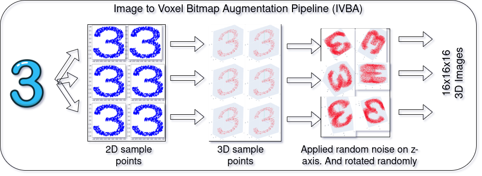
Although I did not had enough experience working with 3D images at that time, I have studied about 3D convolution, Computer Vision, Geometric analysis and how to implement those. I have prior experience with GAN which helped me in this research. A theoretical architecture is given in the below figure and a data generation pipeline (IVBA) is tested and proposed on the next figure.
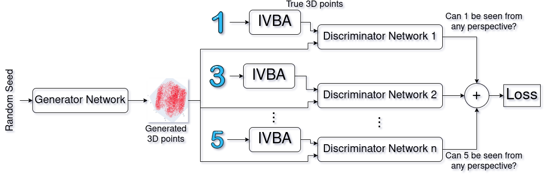
Some examples of the actual implementation is shown at the top of this page.
The actual mathematical explanation can be shown in terms of the original equations with GAN, but with multiple discriminator networks.
\begin{equation}
D = Discriminator
\end{equation}
\begin{equation}
G = Generator
\end{equation}
\begin{equation}
\theta_d = Parameters of discriminator
\end{equation}
\begin{equation}
\theta_g = Parameters of generator
\end{equation}
\begin{equation}
P_z(z) = Input noise distribution
\end{equation}
\begin{equation}
P_{data}(x) = Original data distribution
\end{equation}
\begin{equation}
P_g(x) = Generated distribution
\end{equation}
The Cross-Entropy loss function for the reconstruction process is:
\begin{equation}
\begin{split}
Loss(\hat{y}, y) = y \times log \hat{y} + (1-y) \times log(1-\hat{y})
\end{split}
\end{equation}
So for the whole dataset, it will be:
\begin{equation}
Loss(D(x), 1) = log(D(x)) \
\end{equation}
\begin{equation}
Loss(D(G(z)), 0) = log(1-D(G(z)))
\end{equation}
Objective function of Discriminator networks:
\begin{equation}
\begin{split}
Loss(D)_{min} \longrightarrow max[log(D(x)) + log(1-D(G(z)))]
\end{split}
\end{equation}
Objective function of Generative networks:
\begin{equation}
Loss(G)_{min} \longrightarrow min[log(D(x)) + log(1-D(G(z)))]
\end{equation}
So Overall Objective function will be:
\begin{equation}
min_G max_D [log(D(x)) + log(1 - D(G(z)))]
\end{equation}
Iterations
At each of the iterations, we can see how the reconstruction is actually happening at each iteration.
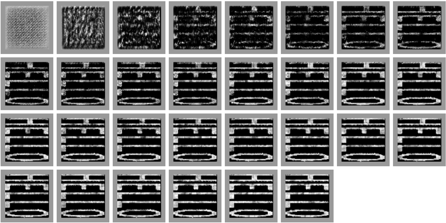


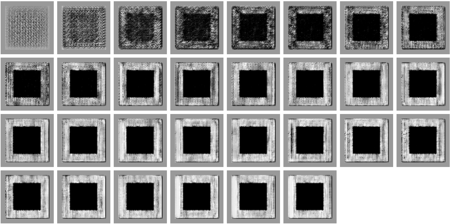
All the corresponding loss values at each iteration can be found in the neptune experiment website.
