Machine Learning Made Easy: Scikit-Learn (Part-1: Basics and Supervised Learning)

Introduction

In this lesson, we will go through some common usages of the powerful and most popular Machine Learning framework, Scikit-Learn. The scikit-Learn library helps all the newcomers to learn more about different Machine Learning practices. It helps the user to achieve the most trivial machine learning tasks in the fewest lines possible. Although Scikit-Learn requires you to learn the very basics of Machine Learning (e.g. model fitting, predicting, cross-validation, etc.), we will learn those in the process of learning this awesome framework.

Installation

To install scikit-learn and scikit-image (a dependency for image processing with scikit-learn, we will use this later), just try the below command in your desired environment/package manager.

1
2
3
4
5
6
7

# pip
pip install -U scikit-learn
pip install -U scikit-image

# Conda
conda install -c conda-forge scikit-learn
conda install scikit-image

The Basics

Scikit-learn (sklearn) tries to divide everything related to Machine Learning into the following categories.

1. Supervised Learning:

   a. Classification Problem

   b. Regression Problem

2. Unsupervised Learning

   a. Density Estimation

   b. Clustering

   c. Dimensionality Reduction

Based on these classifications, sklearn has tried a uniform approach for all the data, transformation, preprocessing, and models. In this lesson, we will only have a look at supervised learning. Let us discuss each of these one by one.

Handling Data with sklearn

Sklearn has a very mature dataset loading and preprocessing end-to-end working methods. It also has a few standard datasets, for instance, the iris and digits datasets for classification and the diabetes dataset for regression. Let us first load the first two datasets.

1
2
3
4

from sklearn import datasets

iris = datasets.load_iris()
digits = datasets.load_digits()

Sklearn datasets are of type Bunch, an internal dataset type for sklearn very similar to a dictionary. You can access the data directly by the attribute data which is a NumPy array. The shape of this array is always of (n_samples, n_features).

Of course, you can use any data from any source. We will discuss how and where to find data in another lesson. Assuming all the data will be a NumPy array, it will work with any function in sklearn.

Alongside learning about Scikit-learn, we will try to create a classification supervised learning algorithm with sklearn only. You will slowly see, how easy it is to create an end-to-end ML pipeline, with sklearn.

Loading Dataset

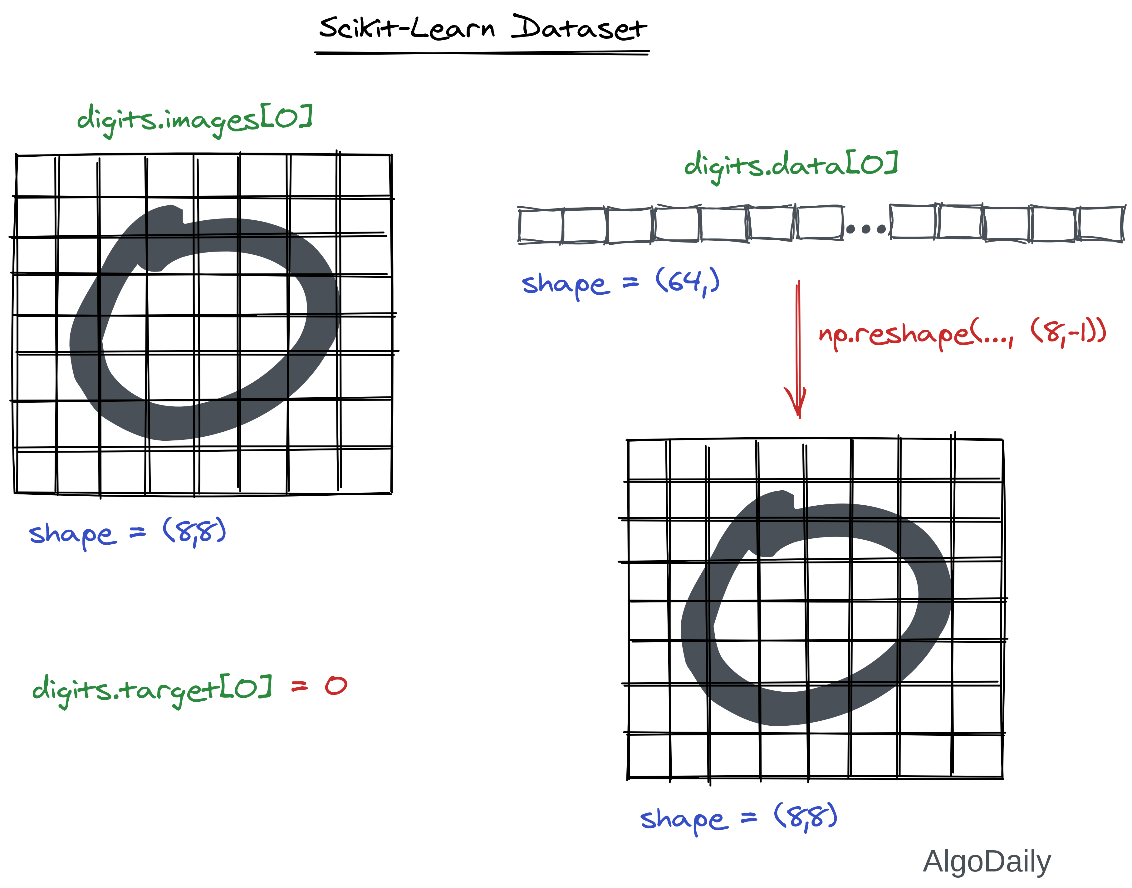
As we can see in the previous example, the digits data is of shape (1797, 64). This means that the data has n_sample=1797 samples, each having n_features=64 features. If you look at the dataset documentation, you will see that it has many attributes. Among them, the most interesting attributes are “data”, “target”, and “images”. Access them in your code and see what each of those are.

 1
 2
 3
 4
 5
 6
 7
 8
 9
10

# Visualize from image attribute
plt.gray() 
plt.matshow(digits.images[0]) # Image of 0
plt.show() 

# Visualize from data attribute
plt.matshow(digits.data[0].reshape(8, -1)) # Image of 0

# The target of the digit
digits.target[0] # 0

Preprocessing with Sklearn

For preprocessing the data, sklearn provides a separate submodule names sklearn.preprocessing. There are about 27 preprocessing functions included in scikit-learn (and still growing). First, we will have a look at the general structure and workflow of how a preprocessing step/function works in sklearn. The typical snippet for data processing goes like this:

 1
 2
 3
 4
 5
 6
 7
 8
 9
10
11
12
13
14
15

# There is no class/function named processor, replace it with an actual processor of sklearn
from sklearn import preprocessing

# Get an instance of processor
processor_instance = preprocessing.Processor()

# Fit and Transform your data separately
processor_instance.fit(data)
transformed_data = processor_instance.transform(data).toarray()

# Or in one step
transformed_data = processor_instance.fit_transform(data).toarray()

# To inverse this process
data = processor_instance.inverse_transform(transformed_data)

There are many types of preprocessing, let us discuss some of the common ones we will use in this lesson. As there are tons of transformation functions, please go ahead and look at the API documentation to learn about all of them.

OneHot Encoding

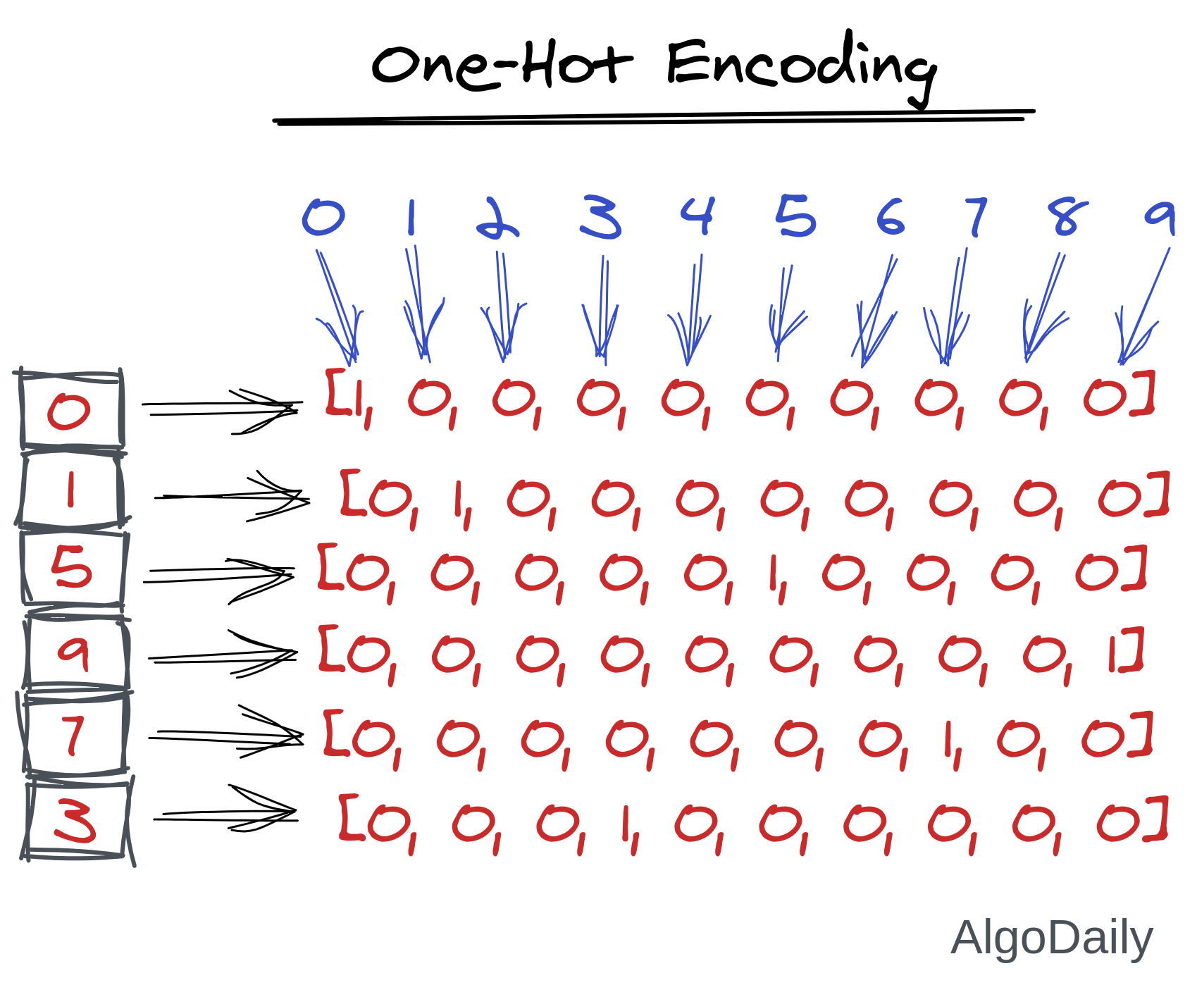
As we were working with the digits dataset, let us transform the target labels into one-hot encoded labels. Here, one-hot encoding means we will assign a binary value for each of the categories of the label/feature.

1
2
3
4

onehot_encoder = preprocessing.OneHotEncoder()
encoded_labels = onehot_encoder.fit_transform(digits.target.reshape(-1, 1)).toarray()

encoded_labels.shape # (n_samples, 10)

Binarization of array

If you want an array to be binary, where all the nonzero values will be turned to 1, you can use the Binarizer preprocessor of sklearn. Without the help of sklearn, you would need to do something like this:

1
2

np_done = digits.data.copy()
np_done[np_done != 0] = 1

But, later you’ll know that this kind of processing is not robust, and you cannot use this is a complete ML pipeline made by sklearn. So, we will use sklearn.preprocessing.Binarizer for this.

1

binary_image = preprocessing.Binarizer().fit_transform(digits.data)

Binarizer will only replace the nonzero values to 1. If you want a more robust binarization like threshold, you can use the preprocessing function binarize directly without instantiating.

1

binary_image = preprocessing.binarize(digits.data, threshold=0.5)

Label Encoding

This preprocessing function is very important as it is used in many different algorithms to process data first. Although we do not need this preprocessing to build our digits classifier because the target is already label encoded, it is worth learning now!

Let’s imagine that our target of the digits object is not given like an array of [0..9]. They are given as a string of names of the digits. See the code below:

1
2
3
4

# Lets think we do not have digits.target at our hand
# Instead, we have "targets" like below

targets = ['one', 'zero', 'one', 'two', 'five', 'three', 'four', 'eight', 'six', 'nine', 'seven']

Then, how do we input this array of string into our model/classifier? We have to change the array, and replace all the values of “one"s into 1, “two"s into 2, and so on. This is what label encoded does.

1
2
3
4
5
6
7
8
9

le = preprocessing.LabelEncoder()

targets_encoded = le.fit_transform(targets)
print(targets_encoded) # [4 9 4 8 1 7 2 0 6 3 5]

# We use targets_encoded in our ML classification

targets_decoded = le.inverse_transform(targets_encoded)
print(targets_decoded) # Same as targets

Remember, the encoded label of values 0..9 are insignificant of the actual labels of the images we know. Here, an image of “1” can be encoded as 5 (because of the internal implementation of sklearn). But it won’t matter as long as all the images of “1” are encoded as 5. We can again inverse_transom to get the actual string again

Feature Scaling and Normalization

Previously, we have done feature scaling using two methods, min-max feature scaling and standardization. We did both of them using only NumPy. For this, we had to remember the equation and implement it every time. Sklearn has built-in preprocessor classes for both of these.

We will use this feature scaling for our digit classification. Note that, currently the range of the data is:

1

print('range is :', digits.data.min(), ',', digits.data.max()) # (0.0 , 16.0)

So we will apply min-max feature scaling on this to make them from 0 to 1. We are also showing the standardization, but as this data does not follow any gaussian distribution, we won’t be using it as a preprocessing step.

As you already know about these scaling methods, let’s just get familiarized with the classes only.

1
2
3
4
5
6
7

# Min-Max scaling
scaler = preprocessing.MinMaxScaler(feature_range=(0, 1), clip=True)
scaled_data = scaler.fit_transform(digits.data)

# Normalization
scaler = preprocessing.StandardScaler()
scaled_data = scaler.fit_transform(digits.data)

Custom Preprocessing Methods

Although sklearn offers tons of different preprocessing methods, we may need something else that is not available. Then, we can easily use preprocessing.FunctionTransformer to build our own preprocessor. This object takes a callable in its constructor which will do our required preprocessing. The callable must take the input X and return an output array whose first dimension must be equal to n_samples. We can also provide another function for the inverse transformation.

For example, there is no preprocessor to apply the log function on the data. We can easily build one ourselves.

1
2

log1p = preprocessing.FunctionTransformer(np.log1p)
logged_data = log1p.transform(digits.data)

Splitting Train and Test

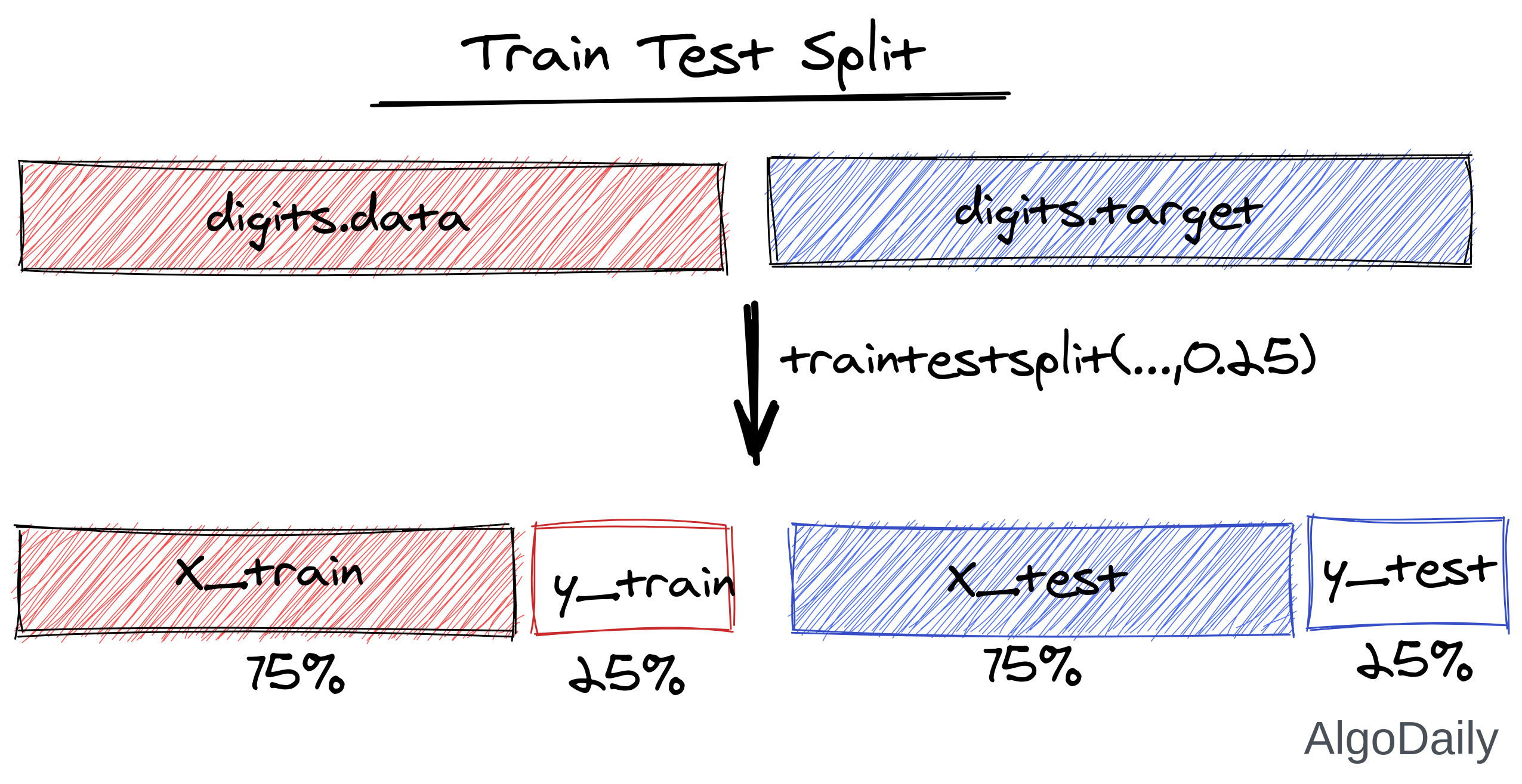
In a previous lesson, we shuffled the dataset along with the target, and then took the first 80% of the data as train, 20% data as cross-validation. We can do all of these with only one line. Let’s split our digits dataset into train and cross-validation.

1
2
3
4

from sklearn.model_selection import train_test_split # Train Test split

# Shuffle and divide the data into two parts, the second one having 25% of the whole data (all with labels).
X_train, X_test, y_train, y_test = train_test_split(digits.data, digits.target, test_size=0.25, random_state=42)

Classification with Sklearn

Now that we know how to load and preprocess the data, we can create several classifiers and train them on the data. Finally, we will also do model evaluation and select the best model with the best parameters.

A model in sklearn is another name for estimator. An estimator for classification is a Python object that implements the methods fit(X, y) and predict(T).

We will try some classifiers and see which one works best. First, let’s start with a Decision Tree classifier. We will use these classifiers as a black box as their mathematical background is quite complex and out of the scope of this series. But you are welcome to look into the details here.

 1
 2
 3
 4
 5
 6
 7
 8
 9
10
11
12
13

from sklearn.tree import DecisionTreeClassifier # Our first classifier
from sklearn.metrics import accuracy_score # To calculate accuracy

# Build the classifier
clf = DecisionTreeClassifier(random_state=0)
# Now train it
clf.fit(X_train, y_train)

# Predict our cross-validation data
pred = clf.predict(X_test)

# Calculate accuracy of the model
print(accuracy_score(pred, y_test)) # 0.8688888888888889

Well, the accuracy is not very bad. Let us see if any other model does better or not.

Another example of an estimator is the class sklearn.svm.SVC, which implements support vector classification. The estimator’s constructor takes as arguments the model’s parameters. For now, we will consider the estimator as a black box:

1
2
3
4
5
6
7

from sklearn import svm
from sklearn.metrics import accuracy_score # To calculate accuracy

clf = svm.SVC(gamma=0.001, C=100.)
clf.fit(X_train, y_train)
pred = clf.predict(X_test)
print(accuracy_score(pred, y_test)) # 0.9911111111111112

Whoa, the accuracy is great! So it seems Support Vector Machine (SVM) classifiers worked better in this dataset. This is done without any preprocessing at all.

Selecting the right model with the right parameters

In the previous section, we used two models for predicting the digits. Decision Tree Classifier and Support Vector Machine. Again in SVM, we used two hyper-parameters, gamma and C. We can certainly tell that SVM is better for classifying this dataset. But there are some scenarios, where only the accuracy of the cross-validation set is not enough to compare two classifiers. Moreover, how are you sure that the value 0.001 for gamma and 100 for C is the best. We could change these hyper-parameters and get even better results.

All of these tasks are part of model evaluation. Every sklearn estimator exposes a score method that can quickly evaluate that classifier. Let’s see how to use it:

1
2
3

clf = svm.SVC(gamma=0.001, C=100.)
clf.fit(X_train, y_train)
clf.score(X_test, y_test)

So, for different values, we could do something like this:

1
2
3
4

for gamma, C in np.array(np.meshgrid([0.0001, 0.001, 0.005, 0.01, 0.1], [10, 50, 100, 200, 500])).T.reshape(-1,2):
    clf = svm.SVC(gamma=gamma, C=C)
    clf.fit(X_train, y_train)
    print(f"Gamma = {gamma}, C = {C} \t| Score: {clf.score(X_test, y_test)}")

Notice how complex it is to get all the combinations of different parameters for the classification score.

Grid Searching

The above implementation complexity can be avoided using the Grid-Search method of Scikit-Learn. We only need to provide the values we want to experiment with, and everything will be taken care of automatically.

 1
 2
 3
 4
 5
 6
 7
 8
 9
10
11
12
13
14
15
16
17
18
19

from sklearn.model_selection import GridSearchCV, cross_val_score

gammas = [0.0001, 0.001, 0.005, 0.01, 0.1]
Cs = [10, 50, 100, 200, 500]

# We are wr
grid_searcher = GridSearchCV(
    estimator=clf,
    param_grid=dict(
        C=Cs,
        gamma=gammas
    ),
    n_jobs=-1
)

grid_searcher.fit(X_train, y_train)        
print("Best Score is ", grid_searcher.best_score_)
print("Best C is ", grid_searcher.best_estimator_.C)
print("Best Gamma is ", grid_searcher.best_estimator_.gamma)

The output is:

1
2
3

Best Score is  0.988861352058378
Best C is  10
Best Gamma is  0.001

Without calculating combinations and running for all combinations in a for loop, we have achieved similar results much easier. With this method, we do not need to go through the result to search for the best score. It is already given to us.

Note that Grid Search of Scikit-Learn is not the same as we manually did in the for-loop. It is much more efficient in many ways. First of all, it does not run the estimator for all the parameter combinations. It applies a grid-search algorithm to slowly reach the optimal combination. For example, if the score of both (0.0005,10) and (0.005,10) for the value of (gamma, C) are worse than (0.001,10), the algorithm will never run it for any other value of gamma. Because 0.001 is found to be the optimal one. Secondly, it uses multiple cores of the CPU to run estimators in parallel which greatly speeds things up.

K-Fold Cross-Validation

Sometimes, a model/classifier works very well on a particular test data but does not work well on other test data. For example, our digit classifier may work well for this test data but may fail to predict correctly if we take the first 20% of data as a test. This is known as the residual problem.

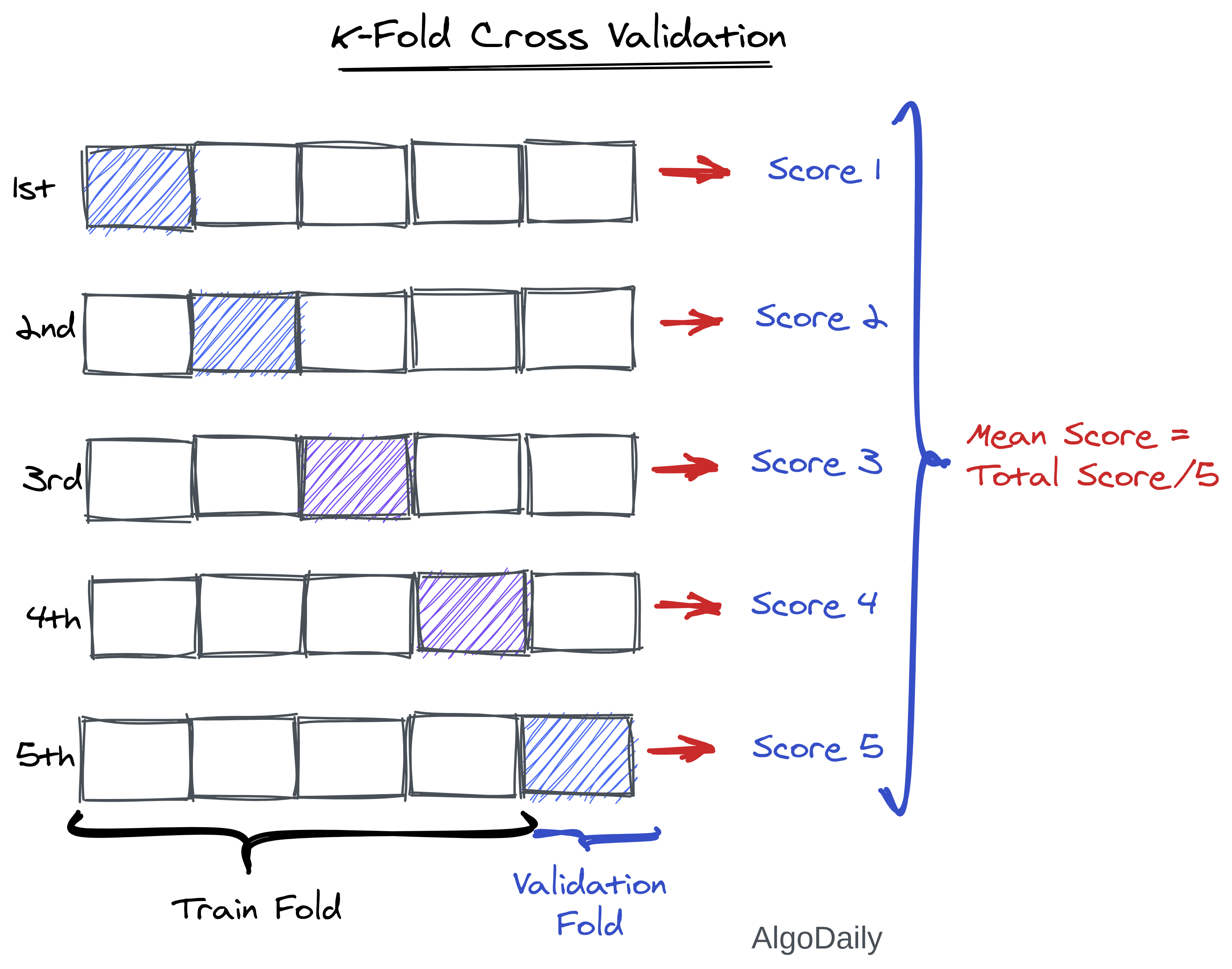
To solve this uncertain accuracy problem, K-Fold Cross Validation is a great method. In K-Fold Cross Validation, the data set is divided into k subsets, and the holdout method is repeated k times. Each time, one of the k subsets is used as the test set and the other k-1 subsets are put together to form a training set. Then the average error across all k trials is computed. The advantage of this method is that it matters less how the data gets divided. Every data point gets to be in a test set exactly once and gets to be in a training set k-1 times. The variance of the resulting estimate is reduced as k is increased. The disadvantage of this method is that the training algorithm has to be rerun from scratch k times, which means it takes k times as much computation to make an evaluation.

Sklearn provides a lot of ways to perform cross-validation in your data. We are showing you only some popular methods here.

 1
 2
 3
 4
 5
 6
 7
 8
 9
10
11
12
13
14

# Loop through K-folds and train yourself
accuracies = []
for train, test in KFold(n_splits=5).split(digits.data, digits.target):
    clf = svm.SVC(gamma=0.001, C=100.)
    clf.fit(digits.data[train], digits.target[train])
    accuracy = clf.score(digits.data[test], digits.target[test])
    accuracies.append(accuracy)
print(accuracies)

# One Liner of the above approach
[svm.SVC(gamma=0.001, C=100.).fit(digits.data[train], digits.target[train]).score(digits.data[test], digits.target[test]) for train, test in KFold(n_splits=5).split(digits.data, digits.target)]

# To become more automated without the loop run by ourselves
cross_val_score(svm.SVC(gamma=0.001, C=100.), digits.data, digits.target, cv=KFold(n_splits=5)) # Get mean to get final result

With these techniques, you can easily compare different estimators and get the best classifier for your dataset.

Solving different dataset problems with different approaches

As of the official guide of Scikit-learn, often the hardest part of solving a machine learning problem can be finding the right estimator for the job. Different estimators are better suited for different types of data and different problems.

The flowchart below is designed to give users a bit of a rough guide on how to approach problems concerning which estimators to try on your data.

End-to-End Pipelines

Suppose you are reading raw data from somewhere, preprocessing it, and then finally training it on a classifier. Maybe you are using that result to input into another classifier? Or you are doing multiple stages of preprocessing. After writing several functions, you want to apply your data to all of those functions. This time, again you will need to call all those functions separately. In the process, you need to maintain the flow order of the data and maintain the matching of shapes of data across different functions.

This sounds a bit cumbersome, right? Sklearn is here again to the rescue. Scikit-Learn has sklearn.pipeline to create one single call to apply all these functions sequentially, providing you what you only care about, the final predictions. In the code snippet below, we are creating a pipeline for our digit classifier and applying it to the test data.

1
2
3
4
5
6
7
8

from sklearn.pipeline import Pipeline

pipe = Pipeline(steps=[
    ('Feature Scaling', preprocessing.MinMaxScaler(feature_range=(0, 1), clip=True)),
    ('SVM', svm.SVC(gamma=0.001, C=10.))
])

cross_val_score(pipe, digits.data, digits.target, cv=KFold(n_splits=5))

Conclusion

In this lesson, we have become familiar with one of the most popular frameworks for machine learning. You will be glad to know that a lot of other ML-based frameworks like TensorFlow, PyTorch share very similar API (e.g. fit, predict). For this, learning scikit-learn after NumPy is the first most important step for any beginners. In the next lesson, we will start learning our final Framework in this series, TensorFlow.