Data Visualization

Introduction

In this lesson, we will introduce two new giant libraries: matplotlib and plotly. There are tons of visualization libraries in python, but matplotlib is the lowest level and most of the other libraries (e.g. seaborn, ggplot, bokeh, etc.) are built only on matplotlib. We are also introducing you to plotly to make you understand what Interactive plots mean. Without any delay, let us get started.

Matplotlib

Let us first install the library matplotlib. We can do it with both pip or conda.

1
2

pip install matplotlib
conda install matplotlib

You can follow the official documentation for matplotlib. But it is quite large, so we are here to summarize everything within only half of this lesson. Also, matplotlib has two kinds of API. The functional and Object API. We will only work with Object API as it is more modern than the other.

Matplotlib graphs your data on Figures (i.e., windows, Jupyter widgets, etc.), each of which can contain one or more Axes (i.e., an area where points can be specified in terms of x-y coordinates, or theta-r in a polar plot, or x-y-z in a 3D plot, etc.). The simplest way of creating a figure with an axes is using pyplot.subplots. We can then use Axes.plot to draw some data on the axes:

1
2
3
4
5
6
7
8

# Matplotlib has a lot of submodules to work with. 
# But in general cases, all we need is the pyplot submodule. 
# By convention, it is always imported as plt
from matplotlib import pyplot as plt

fig, ax = plt.subplots()  # Create a figure containing a single axes.
ax.plot([1, 2, 3, 4], [1, 4, 2, 3])  # Plot some data on the axes.
fig.show()

Now let us understand each part of a full-fledged figure in matplotlib. See the image below:

Matplotlib works best with only NumPy arrays. So if you have something else like a NumPy matrix or pandas dataframe, it is best to convert them to NumPy first. Pandas has a df.values attribute and NumPy has np.asarray(matrix) method to do this.

We only need to work with three types of objects in matplotlib. Try to understand these by seeing the picture below:

So we need to create a figure. Inside that figure, we create several axes. Inside those axes, there will be 2 or 3 axis (like real-life x-axis and y-axis). All of these are done below:

 1
 2
 3
 4
 5
 6
 7
 8
 9
10
11
12
13
14
15
16
17
18
19
20
21
22
23
24
25

x = np.linspace(0, 2, 100)

fig, all_axes = plt.subplots(
    2,3,              # The subplots will be in a grid of size 2x3 
    figsize=(20, 10), # The figure size is 20*80=1600 pixels width and 10*80=800 pixels height 
    dpi=80            # Define the density per pixel (number of pixels in 1 inch)
)  # Create a figure and 6 axes

((axs11, axs12, axs13),(axs21, axs22, axs23)) = all_axes

axs11.plot(x, x**1, label='linear')       # Plot some data on the axes.
axs12.plot(x, x**2, label='quadratic') # Plot more data on the axes...
axs13.plot(x, x**3, label='cubic')     # ... and some more.

axs21.plot(x, x**1, label='linear')     # ... and some more.
axs22.plot(x, x**(1/2), label='quadratic')     # ... and some more.
axs23.plot(x, x**(1/3), label='cubic')     # ... and some more.

for axs in all_axes.reshape(-1):         # Loop through all axes. Here axes are np.array of shape (2,3). We reshape it to 1D.
    axs.set_xlabel('x label')            # Add an x-label to the axes.
    axs.set_ylabel('y label')            # Add a y-label to the axes.
    axs.set_title("Simple Plot")         # Add a title to the axes.
    axs.legend()                         # Add a legend.

fig.show()

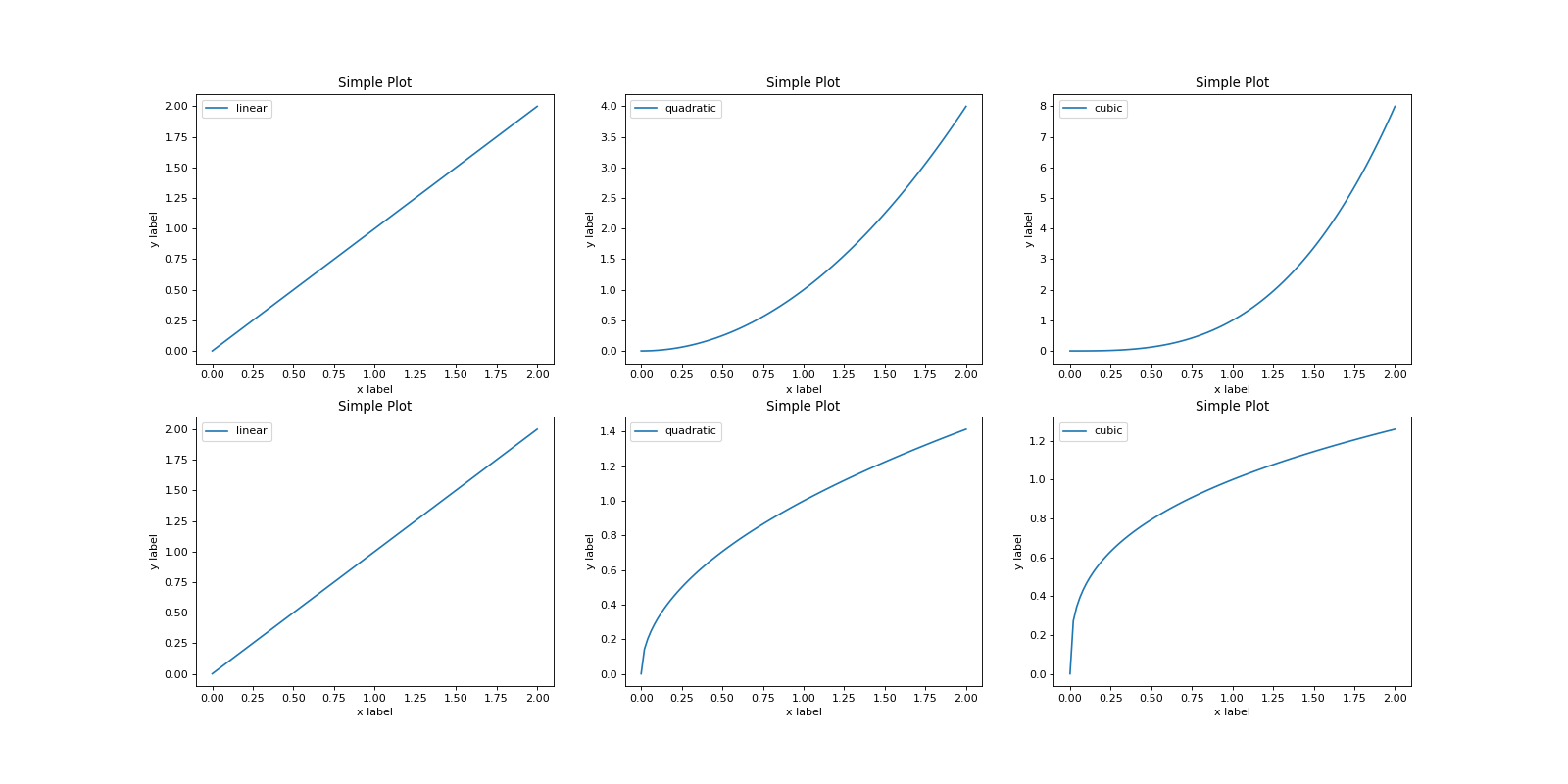
We will go through each type of plot one by one right after we introduce an interactive plot next.

Plotly

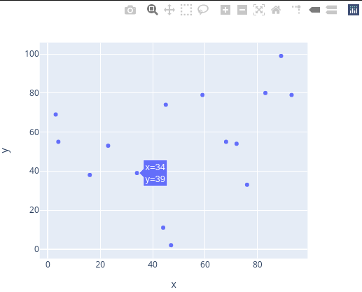
Plotly is a plotting/data visualization library written in Javascript. It is ported to python and used with HTML, JS right inside python. The most amazing feature of plotly is that it helps you create interactive plots. Interactive plots are those plots where you can interact. You can zoom in, filter a subset of the data visualized, and change the scale of any axis. All of these and much more are achievable inside plotly.

The only downside of plotly is its performance. It is reasonably very slow compared to matplotlib as it is manipulating a full-fledged website written with HTML, CSS, and Javascript.

Installing plotly is a little trickier than installing other python libraries. First, install the plotly core library using pip or conda.

1
2
3
4
5

pip install plotly
# or
# The latest version of plotly is not available in the base channel. 
# So we install it from its own channel
conda install plotly -c plotly 

This will install everything required to use plotly. But, if you want to install it into jupyter notebook or jupyter-lab, then you need to install ipywidgets python package.

1
2
3

pip install ipywidgets
# or
conda install ipywidgets

For jupyter-lab, you want to add the jupyterlab extension as well.

1
2

# Only for jupyter-lab
jupyter labextension install jupyterlab-plotly

Mostly, plotly works with Graph Objects and traces inside them. On the other hand, plotly provides a submodule named express. This is a layer above plotly to make common types of plotting much easier. For this lesson, we will only use plotly express for most of the plotting.

Unlike matplotlib, plotly works best with pandas Dataframes. So it is best to create a dataframe from the NumPy array or matrix to visualize with plotly.

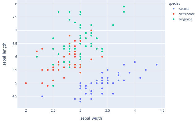
Plotly also has a set of datasets inside the library mostly for demo purposes. Let’s use the iris dataset and plot it with plotly express.

1
2
3
4

import plotly.express as px
df = px.data.iris()
fig = px.scatter(df, x="sepal_width", y="sepal_length", color="species")
fig.show()

Let us start to draw different kinds of plots for different kinds of data using both matplotlib and plotly library.

Types of Plots

There are common types of plots that are well established for different classes of data. Almost all the plotting libraries including matplotlib and plotly have implementations of these types of plots. Let’s discuss that one at a time.

Scatter Plot

Given two continuous features, we can create a plot where the x-axis represents one and the y-axis represents another. Then each of the samples will represent a point on the plot. This is ideal when we want to detect any relational pattern between two features.

Let’s implement this on matplotlib:

1
2
3
4
5
6

import matplotlib.pyplot as plt

x = np.random.randint(0, 100, 15)
y = np.random.randint(0, 100, 15)
plt.scatter(x, y)
plt.show()

The same thing for plotly is:

1
2
3
4
5
6

import plotly.express as px

x = np.random.randint(0, 100, 15)
y = np.random.randint(0, 100, 15)
fig = px.scatter(x=x, y=y)
fig.show()

For the conciseness of the lesson, we will now only write the data generation and plotting part in a single code snippet.

Line Plot

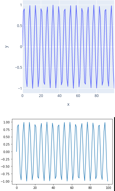
Line plots are very likely to Scatter plots. The main difference in line plots is that the domain of the x-axis will be continuous. Usually, line plots are best to see any kind of function. Also, we can easily detect the trend (upward or downward) in line plots.

Moreover, if you plot multiple functions in the same line plot, you can compare them pretty easily. In later lessons, we will use line plots to see the loss functions, accuracy, etc. with respect to epochs or iterations.

Let us create the same line plot in both matplotlib and plotly.

1
2
3

x = np.arange(100)
plt.plot(x, np.sin(x)) # matplotlib.pyplot
px.line(x=x, y=np.sin(x)) # plotly.express

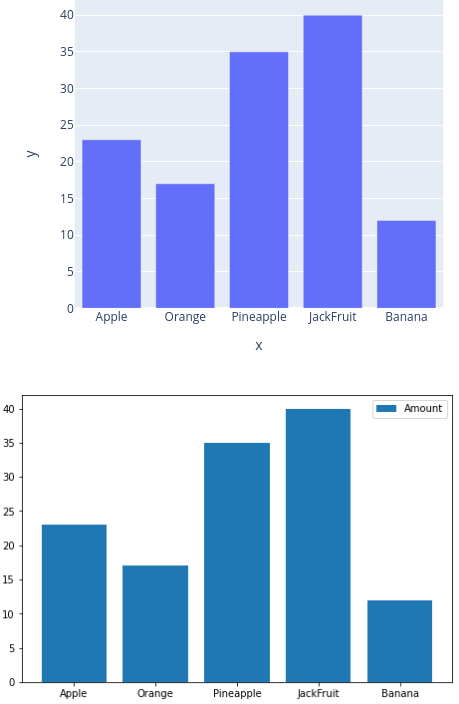
Bar Charts

The bar graphs are used in data comparison where we can measure the changes over a period of time. It can be represented horizontally or vertically. The longer the bar it has the greater the value it contains.

In later lessons, we will use bar charts to see different kinds of categorical variables and compare balance in classes.

 1
 2
 3
 4
 5
 6
 7
 8
 9
10

fruits = ['Apple', 'Orange', 'Pineapple', 'JackFruit', 'Banana']
amount = [23,17,35,40,12]

fig = plt.figure()
ax = fig.add_axes([0,0,1,1]) # [x0, y0, width, height]
ax.bar(fruits,amount)
ax.legend(labels=['Amount'])
fig.show()

px.bar(x=fruits, y=amount)

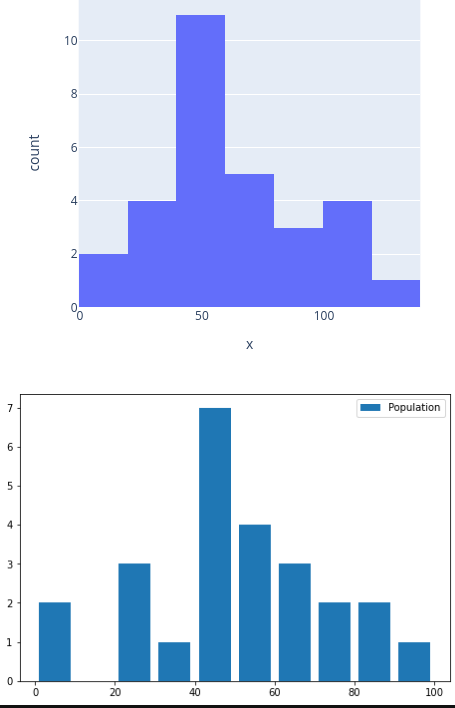
Histogram

The histogram is used where the data is been distributed while the bar graph is used in comparing the two entities. Histograms are preferred during the arrays or data containing the long list. Consider an example where we can plot the age of the population with respect to the bin. The bin refers to the range of values divided into a series of intervals. In the below example bins are created with an interval of 10 which contains the elements from 0 to 9, then 10 to 19, and so on.

 1
 2
 3
 4
 5
 6
 7
 8
 9
10

population_age = [22,55,62,45,21,22,34,42,42,4,2,102,95,85,55,110,120,70,65,55,111,115,80,75,65,54,44,43,42,48]
bins = [0,10,20,30,40,50,60,70,80,90,100]

fig = plt.figure()
ax = fig.add_axes([0,0,1,1]) # [x0, y0, width, height]
ax.hist(population_age,bins=bins, rwidth=0.8)
ax.legend(labels=['Population'])
fig.show()

px.histogram(x=population_age, nbins=11)

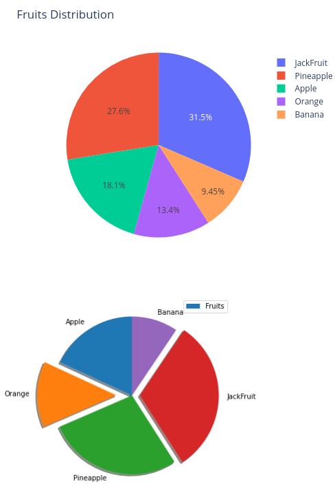
Pie Chart

A pie chart is a circular graph that is divided into segments or slices of pie (Like a Pizza). It is used to represent the percentage or proportional data where each slice of the pie represents a category. This is very similar to Bar chart, but in a circular fashion.

When there is an order defined in the labels, or there are too many labels then we will use Bar charts. And when the label does not have any order, we can use Pie Charts.

We will use Pie Charts for attribute balance checking, categorical data proportion, etc. in a later lesson.

 1
 2
 3
 4
 5
 6
 7
 8
 9
10

fruits = ['Apple', 'Orange', 'Pineapple', 'JackFruit', 'Banana']
amount = [23,17,35,40,12]

fig = plt.figure()
ax = fig.add_axes([0,0,1,1])
ax.pie(amount, labels=fruits, startangle=90,shadow=True,explode=(0,0.2,0,0.1,0))
ax.legend(labels=['Fruits'])
fig.show()

px.pie(values=amount, names=fruits, title='Fruits Distribution')

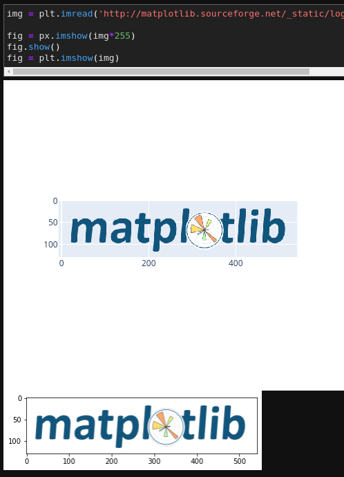
Display Images

Both matplotlib and plotly can also display images, annotate them, show their histogram, and many more things. We will go through this when we introduce CNN (Convolutional Neural Network).

1
2
3
4
5
6
7
8

img = plt.imread('http://matplotlib.sourceforge.net/_static/logo2.png')

# Plotly
fig = px.imshow(img*255)
fig.show()

# matplotlib
plt.imshow(img)

Conclusion

There are numerous ways of visualization of your data. Later, we will also have a look at a clustering dataset, where we will extensively use scatter plots with colors. Till then, try to play around with different types of data. And finally, go through the tutorial of both matplotlib and plotly.