This page looks best with JavaScript enabled

Machine Learning Tutorial - Lesson 11

Lesson 11 out of 12

 ·   ·  ☕ 26 min read · 👀... views
All these tutorial are written by me as a freelancing working for tutorial project AlgoDaily. These has been slightly changed and more lessons after lesson 12 has been added to the actual website. Thanks to Jacob, the owner of AlgoDaily, for letting me author such a wonderful Machine Learning tutorial series. You can sign up there and get a lot of resources related to technical interview preparation.

Real World Deep Neural Network Examples

Introduction

After the last lesson, I hope you have got the primer of how Deep Learning and TensorFlow work. In this lesson, we will use some real-life Deep Learning networks, that are used in production for many different applications. The work needed behind creating and training these models is a lot, and you simply cannot go through all the details of each model in this single lesson. So we will focus more on the application and specialty of these models. We will only load the pre-trained models, and run them on some of our custom images.

Traditional Neural Networks

AlexNET

AlexNet CNN is probably one of the simplest methods to approach understanding deep learning concepts and techniques. This is why this network is the first one I want to introduce to all of you. AlexNet is not a complicated architecture when it is compared with some state-of-the-art CNN architectures that have emerged in more recent years.

Note: We will create a complete Keras pipeline for only this section. As most of the pipelines in Keras are almost the same, the later discussion will only go through the model architecture definition function.

Maybe you are already tired to see the fashion MNIST and IRIS dataset. That’s why we will use a different dataset in this lesson, CIFAR-10 dataset. This can also be found inside the datasets submodule of TensorFlow.

But first things first, we import all the modules we need for the pipeline:

1
2
3
4
5
import numpy as np
import tensorflow as tf
from tensorflow.keras.models import Sequential
from tensorflow.keras import layers
import matplotlib.pyplot as plt

And now we load the training set. CIFAR-10 is a dataset of images of different animals just like the MNIST dataset. But the dataset is larger than MNIST. It contains 50 thousand images for the training set and 10 thousand images for the test set. We will divide the training dataset into two again: for training and validation. The first five thousand images will be for validation, and the later ones will be for training. We can easily do this using NumPy slicing.

1
2
3
4
5
(train_images, train_labels), (test_images, test_labels) = tf.keras.datasets.cifar10.load_data()
CLASS_NAMES= ['airplane', 'automobile', 'bird', 'cat', 'deer', 'dog', 'frog', 'horse', 'ship', 'truck']

validation_images, validation_labels = train_images[:5000], train_labels[:5000]
train_images, train_labels = train_images[5000:], train_labels[5000:]

The most convenient way to train a dataset is through a TensorFlow dataset object as discussed in a previous lesson. So we will convert these NumPy arrays into a TensorFlow dataset using from_tensor_slices method of the Dataset submodule. Finally, we can see the number of images in each division using the cardinality method.

1
2
3
4
5
6
7
8
train_ds = tf.data.Dataset.from_tensor_slices((train_images, train_labels))
test_ds = tf.data.Dataset.from_tensor_slices((test_images, test_labels))
validation_ds = tf.data.Dataset.from_tensor_slices((validation_images, validation_labels))

get_ds_size = lambda ds: tf.data.experimental.cardinality(ds).numpy()
print("Training data size:", get_ds_size(train_ds))
print("Test data size:", get_ds_size(test_ds))
print("Validation data size:", get_ds_size(validation_ds))

The output is:

1
2
3
Training data size: 45000
Test data size: 10000
Validation data size: 5000

Let us take a look at some of the images using matplotlib. We will use the take method to randomly sample some images and display them in subplots.

1
2
3
4
5
6
plt.figure(figsize=(20,20))
for i, (image, label) in enumerate(train_ds.take(5)):
    ax = plt.subplot(5,5,i+1)
    plt.imshow(image)
    plt.title(CLASS_NAMES[label.numpy()[0]])
    plt.axis('off')

cifar

Now comes the preprocessing part. The pixel values of the images are now in the range of 0-255. We need to convert it into a range of -1 to 1. Thanks to the convenience of the Dataset submodule, you can use the per_image_standardization method on the dataset. After resizing it to the model’s desired shape, we shuffle the data and apply a batch size of 32 to train the model.

 1
 2
 3
 4
 5
 6
 7
 8
 9
10
11
12
13
14
15
16
17
18
19
20
def preprocess(image, label):
    # Standardize each images
    image = tf.image.per_image_standardization(image)
    # AlexNET takes input of size (227,227)
    # Resize all images to 277x277
    image = tf.image.resize(image, (227,227))
    return image, label

train_ds = (train_ds
                  .map(preprocess)
                  .shuffle(buffer_size=train_ds_size)
                  .batch(batch_size=32, drop_remainder=True))
test_ds = (test_ds
                  .map(preprocess)
                  .shuffle(buffer_size=train_ds_size)
                  .batch(batch_size=32, drop_remainder=True))
validation_ds = (validation_ds
                  .map(preprocess)
                  .shuffle(buffer_size=train_ds_size)
                  .batch(batch_size=32, drop_remainder=True))

The model architecture contains a set of Convolution-BatchNormalization-MaxPool sets first. Then finally the data is flattened and two fully connected layers of 4096 units are used. As the output is the probability of 10 classes, the final fully connected layer will have 10 units only.

 1
 2
 3
 4
 5
 6
 7
 8
 9
10
11
12
13
14
15
16
17
18
19
20
21
22
23
24
25
26
27
28
model = Sequential([
    layers.Conv2D(filters=96, kernel_size=(11,11), strides=(4,4), activation='relu', input_shape=(227,227,3)),
    layers.BatchNormalization(),
    layers.MaxPool2D(pool_size=(3,3), strides=(2,2)),
    
    layers.Conv2D(filters=256, kernel_size=(5,5), strides=(1,1), activation='relu', padding="same"),
    layers.BatchNormalization(),
    layers.MaxPool2D(pool_size=(3,3), strides=(2,2)),
    
    layers.Conv2D(filters=384, kernel_size=(3,3), strides=(1,1), activation='relu', padding="same"),
    layers.BatchNormalization(),
    
    layers.Conv2D(filters=384, kernel_size=(3,3), strides=(1,1), activation='relu', padding="same"),
    layers.BatchNormalization(),
    
    layers.Conv2D(filters=256, kernel_size=(3,3), strides=(1,1), activation='relu', padding="same"),
    layers.BatchNormalization(),
    layers.MaxPool2D(pool_size=(3,3), strides=(2,2)),
    
    layers.Flatten(),
    layers.Dense(4096, activation='relu'),
    layers.Dropout(0.5),
    
    layers.Dense(4096, activation='relu'),
    layers.Dropout(0.5),
    layers.Dense(10, activation='softmax')
])
model.summary()

For training the model, we can use both Categorical Crossentropy or Sparse Categorical CrossEntropy as the loss function. But using only Categorical cross-entropy will lead us to another step (converting the labels to one-hot encoding). So we will use the sparse one as loss function. The optimizer is the Stochastic Gradient Descent algorithm.

1
model.compile(loss='sparse_categorical_crossentropy', optimizer=tf.optimizers.SGD(learning_rate=0.001), metrics=['accuracy'])

We can now start the training with the fit method on the model.

1
2
3
4
5
6
model.fit(
    train_ds,
    epochs=50,
    validation_data=validation_ds,
    validation_freq=1,
)

Note: This will take a lot of time depending on the machine you are running on. Also if you are low on available memory in your computer, your system may get stuck. Alternatively, you can run a notebook on Google Colab or Kaggle using GPU for free.

To evaluate the model, we can run the evaluate method on the test_ds set.

1
np.mean(model.evaluate(test_ds))
1
2
312/312 [==============================] - 8s 27ms/step - loss: 0.9814 - accuracy: 0.7439
0.8626266404836566

So the mean accuracy on the test set is 86.26%. That is actually good for this old neural network created in 2012.

You Only Look Once (YOLO)

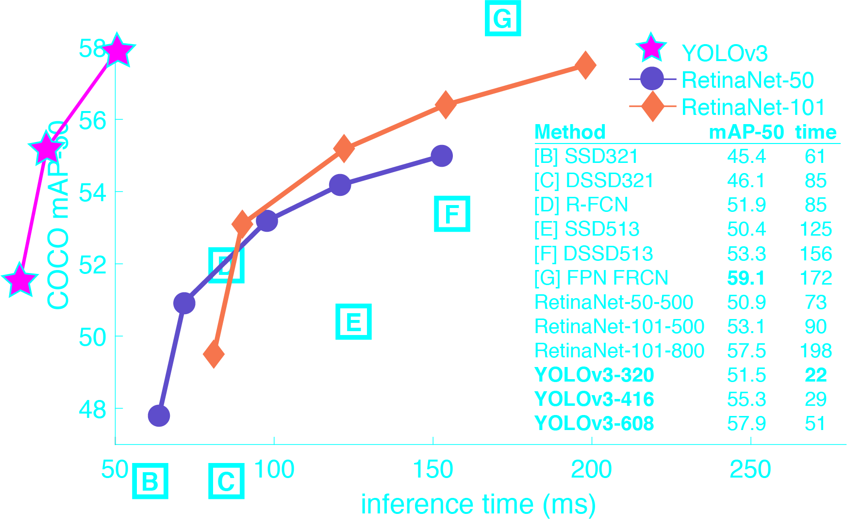
The first model we will try is the YOLO object detection model. This is a model where you can give the image and it will detect a lot of objects for you. The first Yolo model (Yolo V1) could detect 80 real-world objects. YOLO is a state-of-the-art, real-time object detection system. On a Pascal Titan X, it processes images at 30 FPS and has an mAP of 57.9% on COCO test-dev.

The major advantage of YOLO is that it is very fast. Unlike other Classifier based neural networks, YOLO applies image classification on multiple regions in parallel with the help of GPU, and if an object is detected, it uses an object classifier to classify it.

yoloperf

There is a lot of implementation out there for YOLO. The original code for darknet can be used with OpenCV’s DNN module. But we will use a much simpler version by Anushka Dhiman. Although I have no affiliation with any of the persons’ repositories, I only select these because I found these the easiest to use. Her repository supports TensorFlow 2 and is up-to-date with Yolo v3. Let us first download the code and set up the environment.

 1
 2
 3
 4
 5
 6
 7
 8
 9
10
git clone https://github.com/anushkadhiman/YOLOv3-TensorFlow-2.x.git
cd YOLOv3-TensorFlow-2.x

pip install -r ./requirements.txt

# yolov3
wget -P model_data https://pjreddie.com/media/files/yolov3.weights

# yolov3-tiny
wget -P model_data https://pjreddie.com/media/files/yolov3-tiny.weights

There are two YOLO models: yolov3 is the large model with the highest accuracy, and yolov3-tiny is designed to have higher FPS but a little less accuracy. We will try the regular yolov3. To use this on an image, there is a function names detect_image in the utils file. All we need to do is load the model with Load_Yolo_model and then use that function on the image.

1
2
3
4
5
6
7
import cv2
from yolov3.utils import detect_image, detect_realtime, detect_video, Load_Yolo_model, detect_video_realtime_mp
from yolov3.configs import YOLO_INPUT_SIZE

image_path   = "your_image.jpg"
yolo = Load_Yolo_model()
detect_image(yolo, image_path, "detect.jpg", input_size=YOLO_INPUT_SIZE, show=True, rectangle_colors=(255,0,0))

If you want to run the object detection on a video file, then you can use detect_video function.

1
detect_video(yolo, your_video_path, "", input_size=YOLO_INPUT_SIZE, show=False, rectangle_colors=(255,0,0))

Finally, you can also use your primary webcam to apply object detection live.

1
detect_realtime(yolo, '', input_size=YOLO_INPUT_SIZE, show=True, rectangle_colors=(255, 0, 0))

Let us now get a little deep into the implementation of the neural network. The model architecture in python is given below. Yes, it is huge. Most of the established deep learning networks are like this.

  1
  2
  3
  4
  5
  6
  7
  8
  9
 10
 11
 12
 13
 14
 15
 16
 17
 18
 19
 20
 21
 22
 23
 24
 25
 26
 27
 28
 29
 30
 31
 32
 33
 34
 35
 36
 37
 38
 39
 40
 41
 42
 43
 44
 45
 46
 47
 48
 49
 50
 51
 52
 53
 54
 55
 56
 57
 58
 59
 60
 61
 62
 63
 64
 65
 66
 67
 68
 69
 70
 71
 72
 73
 74
 75
 76
 77
 78
 79
 80
 81
 82
 83
 84
 85
 86
 87
 88
 89
 90
 91
 92
 93
 94
 95
 96
 97
 98
 99
100
101
102
103
104
105
106
107
108
109
110
111
112
113
114
115
116
117
118
119
120
121
122
123
124
125
126
127
128
129
130
131
132
133
134
135
136
137
138
139
140
141
142
143
144
145
146
147
148
149
150
151
from keras.layers import Conv2D
from keras.layers import Input
from keras.layers import BatchNormalization
from keras.layers import LeakyReLU
from keras.layers import ZeroPadding2D
from keras.layers import UpSampling2D
from keras.layers.merge import add, concatenate
from keras.models import Model

def convolution_block(x, convs, skip=True):
    count = 0
    for conv in convs:
        if count == (len(convs) - 2) and skip:
            skip_connection = x
        count += 1
        # The model is designed with only left and top padding
        if conv['stride'] > 1: x = ZeroPadding2D(((1,0),(1,0)))(x)
        x = Conv2D(conv['filter'],
                   conv['kernel'],
                   strides=conv['stride'],
                   padding='valid' if conv['stride'] > 1 else 'same', 
                   name='conv_' + str(conv['layer_idx']),
                   use_bias=False if conv['bnorm'] else True)(x)
        if conv['bnorm']:
            x = BatchNormalization(
                epsilon=0.001, 
                name='bnorm_' + str(conv['layer_idx'])
            )(x)
        if conv['leaky']:
            x = LeakyReLU(
                alpha=0.1, 
                name='leaky_' + str(conv['layer_idx'])
            )(x)
    return add([skip_connection, x]) if skip else x

def make_yolov3_model():
    input_image = Input(shape=(None, None, 3))
    # Layer  0 => 4
    x = convolution_block(input_image, [
        {'filter': 32, 'kernel': 3, 'stride': 1, 'bnorm': True, 'leaky': True, 'layer_idx': 0},
        {'filter': 64, 'kernel': 3, 'stride': 2, 'bnorm': True, 'leaky': True, 'layer_idx': 1},
        {'filter': 32, 'kernel': 1, 'stride': 1, 'bnorm': True, 'leaky': True, 'layer_idx': 2},
        {'filter': 64, 'kernel': 3, 'stride': 1, 'bnorm': True, 'leaky': True, 'layer_idx': 3}
    ])
    # Layer  5 => 8
    x = convolution_block(x, [
        {'filter': 128, 'kernel': 3, 'stride': 2, 'bnorm': True, 'leaky': True, 'layer_idx': 5},
        {'filter':  64, 'kernel': 1, 'stride': 1, 'bnorm': True, 'leaky': True, 'layer_idx': 6},
        {'filter': 128, 'kernel': 3, 'stride': 1, 'bnorm': True, 'leaky': True, 'layer_idx': 7}
    ])
    # Layer  9 => 11
    x = convolution_block(x, [
        {'filter':  64, 'kernel': 1, 'stride': 1, 'bnorm': True, 'leaky': True, 'layer_idx': 9},
        {'filter': 128, 'kernel': 3, 'stride': 1, 'bnorm': True, 'leaky': True, 'layer_idx': 10}
    ])
    # Layer 12 => 15
    x = convolution_block(x, [
        {'filter': 256, 'kernel': 3, 'stride': 2, 'bnorm': True, 'leaky': True, 'layer_idx': 12},
        {'filter': 128, 'kernel': 1, 'stride': 1, 'bnorm': True, 'leaky': True, 'layer_idx': 13},
        {'filter': 256, 'kernel': 3, 'stride': 1, 'bnorm': True, 'leaky': True, 'layer_idx': 14}
    ])
    # Layer 16 => 36
    for i in range(7):
        x = convolution_block(x, [
            {'filter': 128, 'kernel': 1, 'stride': 1, 'bnorm': True, 'leaky': True, 'layer_idx': 16+i*3},
            {'filter': 256, 'kernel': 3, 'stride': 1, 'bnorm': True, 'leaky': True, 'layer_idx': 17+i*3}
        ])
    # There is a skip from this layer to the last layer. So storing x
    skip_36 = x
    # Layer 37 => 40
    x = convolution_block(x, [
        {'filter': 512, 'kernel': 3, 'stride': 2, 'bnorm': True, 'leaky': True, 'layer_idx': 37},
        {'filter': 256, 'kernel': 1, 'stride': 1, 'bnorm': True, 'leaky': True, 'layer_idx': 38},
        {'filter': 512, 'kernel': 3, 'stride': 1, 'bnorm': True, 'leaky': True, 'layer_idx': 39}
    ])
    # Layer 41 => 61
    for i in range(7):
        x = convolution_block(x, [
            {'filter': 256, 'kernel': 1, 'stride': 1, 'bnorm': True, 'leaky': True, 'layer_idx': 41+i*3},
            {'filter': 512, 'kernel': 3, 'stride': 1, 'bnorm': True, 'leaky': True, 'layer_idx': 42+i*3}
        ])
    skip_61 = x
    # Layer 62 => 65
    x = convolution_block(x, [
        {'filter': 1024, 'kernel': 3, 'stride': 2, 'bnorm': True, 'leaky': True, 'layer_idx': 62},
        {'filter':  512, 'kernel': 1, 'stride': 1, 'bnorm': True, 'leaky': True, 'layer_idx': 63},
        {'filter': 1024, 'kernel': 3, 'stride': 1, 'bnorm': True, 'leaky': True, 'layer_idx': 64}
    ])
    # Layer 66 => 74
    for i in range(3):
        x = convolution_block(x, [
            {'filter':  512, 'kernel': 1, 'stride': 1, 'bnorm': True, 'leaky': True, 'layer_idx': 66+i*3},
            {'filter': 1024, 'kernel': 3, 'stride': 1, 'bnorm': True, 'leaky': True, 'layer_idx': 67+i*3}
        ])
    # Layer 75 => 79
    x = convolution_block(x, [
        {'filter':  512, 'kernel': 1, 'stride': 1, 'bnorm': True, 'leaky': True, 'layer_idx': 75},
        {'filter': 1024, 'kernel': 3, 'stride': 1, 'bnorm': True, 'leaky': True, 'layer_idx': 76},
        {'filter':  512, 'kernel': 1, 'stride': 1, 'bnorm': True, 'leaky': True, 'layer_idx': 77},
        {'filter': 1024, 'kernel': 3, 'stride': 1, 'bnorm': True, 'leaky': True, 'layer_idx': 78},
        {'filter':  512, 'kernel': 1, 'stride': 1, 'bnorm': True, 'leaky': True, 'layer_idx': 79}
    ], skip=False)
    # Layer 80 => 82
    yolo_82 = convolution_block(x, [
        {'filter': 1024, 'kernel': 3, 'stride': 1, 'bnorm': True,  'leaky': True,  'layer_idx': 80},
        {'filter':  255, 'kernel': 1, 'stride': 1, 'bnorm': False, 'leaky': False, 'layer_idx': 81}
    ], skip=False)
    # Layer 83 => 86
    x = convolution_block(x, [
        {'filter': 256, 'kernel': 1, 'stride': 1, 'bnorm': True, 'leaky': True, 'layer_idx': 84}
    ], skip=False)

    x = UpSampling2D(2)(x)
    x = concatenate([x, skip_61])

    # Layer 87 => 91
    x = convolution_block(x, [
        {'filter': 256, 'kernel': 1, 'stride': 1, 'bnorm': True, 'leaky': True, 'layer_idx': 87},
        {'filter': 512, 'kernel': 3, 'stride': 1, 'bnorm': True, 'leaky': True, 'layer_idx': 88},
        {'filter': 256, 'kernel': 1, 'stride': 1, 'bnorm': True, 'leaky': True, 'layer_idx': 89},
        {'filter': 512, 'kernel': 3, 'stride': 1, 'bnorm': True, 'leaky': True, 'layer_idx': 90},
        {'filter': 256, 'kernel': 1, 'stride': 1, 'bnorm': True, 'leaky': True, 'layer_idx': 91}
    ], skip=False)

    # Layer 92 => 94
    yolo_94 = convolution_block(x, [
        {'filter': 512, 'kernel': 3, 'stride': 1, 'bnorm': True,  'leaky': True,  'layer_idx': 92},
        {'filter': 255, 'kernel': 1, 'stride': 1, 'bnorm': False, 'leaky': False, 'layer_idx': 93}
    ], skip=False)

    # Layer 95 => 98
    x = convolution_block(x, [
        {'filter': 128, 'kernel': 1, 'stride': 1, 'bnorm': True, 'leaky': True,   'layer_idx': 96}
    ], skip=False)

    x = UpSampling2D(2)(x)
    x = concatenate([x, skip_36])

    # Layer 99 => 106
    yolo_106 = convolution_block(x, [
        {'filter': 128, 'kernel': 1, 'stride': 1, 'bnorm': True,  'leaky': True,  'layer_idx': 99},
        {'filter': 256, 'kernel': 3, 'stride': 1, 'bnorm': True,  'leaky': True,  'layer_idx': 100},
        {'filter': 128, 'kernel': 1, 'stride': 1, 'bnorm': True,  'leaky': True,  'layer_idx': 101},
        {'filter': 256, 'kernel': 3, 'stride': 1, 'bnorm': True,  'leaky': True,  'layer_idx': 102},
        {'filter': 128, 'kernel': 1, 'stride': 1, 'bnorm': True,  'leaky': True,  'layer_idx': 103},
        {'filter': 256, 'kernel': 3, 'stride': 1, 'bnorm': True,  'leaky': True,  'layer_idx': 104},
        {'filter': 255, 'kernel': 1, 'stride': 1, 'bnorm': False, 'leaky': False, 'layer_idx': 105}
    ], skip=False)

    model = Model(input_image, [yolo_82, yolo_94, yolo_106])
    return model

Training the model will literally take days if you are planing are planning to train it on a large dataset like Microsoft COCO. There is a total of 62001757 parameters you need to pass through when feeding forward.

VGG Network

Named after Visual Geometry Group, Oxford University, the VGG network is based on repeatable blocks named VGG-blocks. These are groups of convolutional layers that use small filters and max pooling layers. Assuming that you already can readout a code and understand the neural network architecture, I am giving the python code for VGG_Block without describing it:

1
2
3
4
5
def vgg_block(layer_in, n_filters, n_conv):
	for _ in range(n_conv):
    layer_in = Conv2D(n_filters, (3,3), padding='same', activation='relu')(layer_in)
	layer_in = MaxPooling2D((2,2), strides=(2,2))(layer_in)
	return layer_in

You can use VGG blocks in any of your models because they are so simple and effective. In the below example the first two blocks have two convolutional layers with 64 and 128 filters respectively, the third block has four convolutional layers with 256 filters. This is a common usage of VGG blocks where the number of filters is increased with the depth of the model.

1
2
3
4
5
6
# We are using functional API just like the previous YOLO implementation
visible = Input(shape=(256, 256, 3))
layer = vgg_block(visible, 64, 2)
layer = vgg_block(layer, 128, 2)
layer = vgg_block(layer, 256, 4)
model = Model(inputs=visible, outputs=layer)

The summary of the model is like this:

 1
 2
 3
 4
 5
 6
 7
 8
 9
10
11
12
13
14
15
16
17
18
19
20
21
22
23
24
25
26
27
28
29
30
31
_________________________________________________________________
Layer (type)                 Output Shape              Param #
=================================================================
input_1 (InputLayer)         (None, 256, 256, 3)       0
_________________________________________________________________
conv2d_1 (Conv2D)            (None, 256, 256, 64)      1792
_________________________________________________________________
conv2d_2 (Conv2D)            (None, 256, 256, 64)      36928
_________________________________________________________________
max_pooling2d_1 (MaxPooling2 (None, 128, 128, 64)      0
_________________________________________________________________
conv2d_3 (Conv2D)            (None, 128, 128, 128)     73856
_________________________________________________________________
conv2d_4 (Conv2D)            (None, 128, 128, 128)     147584
_________________________________________________________________
max_pooling2d_2 (MaxPooling2 (None, 64, 64, 128)       0
_________________________________________________________________
conv2d_5 (Conv2D)            (None, 64, 64, 256)       295168
_________________________________________________________________
conv2d_6 (Conv2D)            (None, 64, 64, 256)       590080
_________________________________________________________________
conv2d_7 (Conv2D)            (None, 64, 64, 256)       590080
_________________________________________________________________
conv2d_8 (Conv2D)            (None, 64, 64, 256)       590080
_________________________________________________________________
max_pooling2d_3 (MaxPooling2 (None, 32, 32, 256)       0
=================================================================
Total params: 2,325,568
Trainable params: 2,325,568
Non-trainable params: 0
_________________________________________________________________

After building the model, all the other works are pretty much the same. You compile the model with an optimizer, fix learning_rate, batch_size, epochs and other hyperparameters. Then fit the model on a dataset.

Inception Model

inceptionmovie

The inception model was first introduced to the GoogLeNet model back in the 2015 paper. You will be amazed it is still one of the most powerful neural networks out there. Like the VGG model, the inception model also has an inception module which is a block of parallel convolutional layers with different sized filters and a and 3×3 max-pooling layer. The results of all the layers are then concatenated into one layer.

 1
 2
 3
 4
 5
 6
 7
 8
 9
10
11
def inception_module(layer_in, f1, f2, f3):
  # Kernel size increasing at each layer
	conv1 = Conv2D(f1, (1,1), padding='same', activation='relu')(layer_in)
	conv3 = Conv2D(f2, (3,3), padding='same', activation='relu')(layer_in)
	conv5 = Conv2D(f3, (5,5), padding='same', activation='relu')(layer_in)

	pool = MaxPooling2D((3,3), strides=(1,1), padding='same')(layer_in)

	# concatenate filters, assumes filters/channels last
	layer_out = concatenate([conv1, conv3, conv5, pool], axis=-1)
	return layer_out

The function takes the previous layer as input and the kernels for the 3 convolutional layers in an inception module. The concatenated form of these 3 layers is then returned to you for further use.

The rest are the same as VGG network. You need to create a model with multiple linear inception modules in it. As you can see, the model building and summary are just boilerplate codes. The interesting part is the network module layer. This is true for most of the models we will see today.

Residual Model

Residual Model or ResNET is also developed by Google which uses loopback residual blocks. A residual block contains two convolutional layers with the same number of kernels and a small filter size where the output of the second layer is added with the input to the first layer.

 1
 2
 3
 4
 5
 6
 7
 8
 9
10
def residual_module(layer_in, n_filters):
	# conv1
	conv1 = Conv2D(n_filters, (3,3), padding='same', activation='relu', kernel_initializer='he_normal')(layer_in)
	# conv2
	conv2 = Conv2D(n_filters, (3,3), padding='same', activation='linear', kernel_initializer='he_normal')(conv1)
	# add filters, assumes filters/channels last
	layer_out = add([conv2, layer_in])
	# activation function
	layer_out = Activation('relu')(layer_out)
	return layer_out

Keep in mind that you need to be careful about the number of filters in the input and output layer. If they do not match, you will most like get an error. The residual network uses one kind of skip connection, which is the unique part of this architecture. In many cases, a lot of primitive features in the network are lost if the model is too deep. Residual network solves this problem with skip connection. The later layers of the model can select them if it needs the output of the layer that is closer to the image, or the previous layer.

Generative Adversarial networks

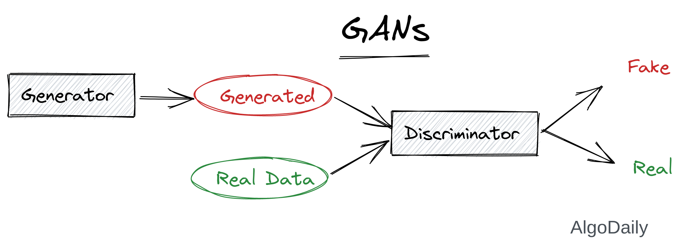
Generative Adversarial Networks (GANs) are one of the most interesting ideas in computer science today. Two models are trained simultaneously by an adversarial process. A generator (“the artist”) learns to create images that look real, while a discriminator (“the art critic”) learns to tell real images apart from fakes.

The main equation upon which the model is built on is given below:

$$min_G max_D (V_{GAN}(D,G) = E_{x ~ P_{data(x)}} [logD(x)] + E_{z~P_z(z)}[log(1-D(G(z)))]$$

To keep it simple, these are the points you need to keep in mind:

  1. Generator takes a random seed and generates a sample
  2. Discriminator takes an image and tries to detect if that image is from a specific distribution (from the actual dataset).
  3. Discriminator is trained on 2 types of images:
    1. Generator generated image with label 0.
    2. An image from the dataset with label 1.

GAN

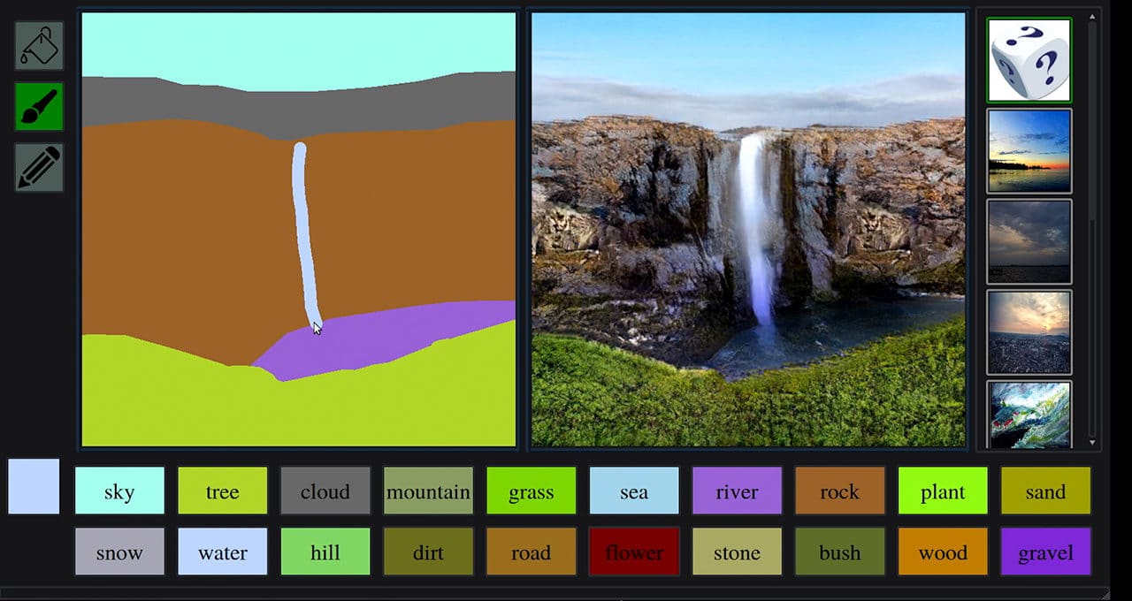
GAN is famous for creating AMAZING original photos out of an existing dataset. Below is an image is taken from NVidia, where you can draw anything and it will be transformed into a photorealistic photo of nature.

nvidia-mountain

TensorFlow’s official website has an intuitive guide of how to implement it on TensorFlow. We will follow that guide, but make the code even simpler so you have no problem understanding it. You already understand that we need to design two models for GAN. First, let’s import everything and take the MNIST dataset as an example. GAN is an unsupervised learning model, so we do not need any labels for our data.

Import what we need:

1
2
3
4
5
import matplotlib.pyplot as plt
import numpy as np
import tensorflow as tf
from tensorflow.keras import layers
import time

And load the data:

1
(train_images, train_labels), (_, _) = tf.keras.datasets.mnist.load_data()

We will create a model where the discriminator will take each image of shape (28,28,1). So the generator has to predict a shape of the same. It can take any size of seed as input, but we will use a linear data of 100 random numbers. Lets reshape and preprocess (simple standardization) the data:

1
2
3
4
# create a grayscale channel which is required for input
train_images = train_images.reshape(train_images.shape[0], 28, 28, 1).astype('float32')
# Normalize the images to [-1, 1]. Previous range was [0,255]
train_images = (train_images - 127.5) / 127.5

Now define some hyperparameters. We will use these variables throughout the code. The names are all self-explanatory

1
2
3
EPOCHS = 50
noise_dim = 100 # seed for generator
BATCH_SIZE = 256

Convert the dataset into a tensorflow dataset:

1
train_dataset = tf.data.Dataset.from_tensor_slices(train_images).shuffle(60000).batch(BATCH_SIZE)

To create the generator model we will start with the noise of shape (100,). After a Dense layer, we reshape the model to a 3D shape to match with the image. The height and width will be 7, and the number of channels will be 256. Later we use a layer named transposed convolution, which is basically the opposite of convolution. The rest are almost the same as any other trivial model.

 1
 2
 3
 4
 5
 6
 7
 8
 9
10
11
12
13
14
15
16
17
18
19
20
21
22
23
24
25
26
27
28
29
30
31
32
33
34
35
36
37
38
39
40
41
def make_generator_model():
    model = tf.keras.Sequential()
    model.add(layers.Dense(7*7*256, use_bias=False, input_shape=(noise_dim,)))
    model.add(layers.BatchNormalization())
    model.add(layers.LeakyReLU())

    model.add(layers.Reshape((7, 7, 256)))
    assert model.output_shape == (None, 7, 7, 256)  # None is the batch size

    model.add(layers.Conv2DTranspose(128, (5, 5), strides=(1, 1), padding='same', use_bias=False))
    assert model.output_shape == (None, 7, 7, 128)
    model.add(layers.BatchNormalization())
    model.add(layers.LeakyReLU())

    model.add(layers.Conv2DTranspose(64, (5, 5), strides=(2, 2), padding='same', use_bias=False))
    assert model.output_shape == (None, 14, 14, 64)
    model.add(layers.BatchNormalization())
    model.add(layers.LeakyReLU())

    model.add(layers.Conv2DTranspose(1, (5, 5), strides=(2, 2), padding='same', use_bias=False, activation='tanh'))
    
    # The output must match the dataset images
    assert model.output_shape == (None, 28, 28, 1)

    return model

def make_discriminator_model():
    model = tf.keras.Sequential()
    model.add(layers.Conv2D(64, (5, 5), strides=(2, 2), padding='same',
                                     input_shape=[28, 28, 1]))
    model.add(layers.LeakyReLU())
    model.add(layers.Dropout(0.3))

    model.add(layers.Conv2D(128, (5, 5), strides=(2, 2), padding='same'))
    model.add(layers.LeakyReLU())
    model.add(layers.Dropout(0.3))

    model.add(layers.Flatten())
    model.add(layers.Dense(1))

    return model

The loss function is the first interesting thing to look at in a GAN. The generator will always be told that its fake inputs are 0 so that it tries to generate better results. The loss of the generator will depend on the output of the discriminator. There will be a lower loss if the discriminator predicts a value close to 1, and 0 otherwise.

For the discriminator, the loss is more straightforward. If the image is from an actual dataset, then the loss is 1. And if the images are coming from the generator, the loss is 0.

Finally, we will use the Adam optimizer with a very small learning rate in the example.

 1
 2
 3
 4
 5
 6
 7
 8
 9
10
11
12
13
cross_entropy = tf.keras.losses.BinaryCrossentropy(from_logits=True)

def generator_loss(fake_output):
    return cross_entropy(tf.ones_like(fake_output), fake_output)

def discriminator_loss(real_output, fake_output):
    real_loss = cross_entropy(tf.ones_like(real_output), real_output)
    fake_loss = cross_entropy(tf.zeros_like(fake_output), fake_output)
    total_loss = real_loss + fake_loss
    return total_loss

generator_optimizer = tf.keras.optimizers.Adam(1e-4)
discriminator_optimizer = tf.keras.optimizers.Adam(1e-4)

The second interesting part of GAN is its training loop. As there are two networks dependent on each other and will be trained simultaneously, the fit method will not work here. We will need to create a custom training loop. While feed forwarding, we keep track of the gradients of each parameter in a GradientTape (separate for each model). After feed forwarding both models, we apply the gradient of loss to both models’ weights.

Note that the training function will need to be compiled so that TensorFlow can build the computation graph first. This helps to speed up the training process and run the function on different devices.

 1
 2
 3
 4
 5
 6
 7
 8
 9
10
11
12
13
14
15
16
17
18
19
# This annotation tells tensorflow to compile the function for training in a device (GPU)
@tf.function
def train_step(images):
    noise = tf.random.normal([BATCH_SIZE, noise_dim])

    with tf.GradientTape() as gen_tape, tf.GradientTape() as disc_tape:
        generated_images = generator(noise, training=True)

        real_output = discriminator(images, training=True)
        fake_output = discriminator(generated_images, training=True)

        gen_loss = generator_loss(fake_output)
        disc_loss = discriminator_loss(real_output, fake_output)

    gradients_of_generator = gen_tape.gradient(gen_loss, generator.trainable_variables)
    gradients_of_discriminator = disc_tape.gradient(disc_loss, discriminator.trainable_variables)

    generator_optimizer.apply_gradients(zip(gradients_of_generator, generator.trainable_variables))
    discriminator_optimizer.apply_gradients(zip(gradients_of_discriminator, discriminator.trainable_variables))

Now that everything is set, we can run several epochs and provide a batch of images to the train_step function.

 1
 2
 3
 4
 5
 6
 7
 8
 9
10
generator = make_generator_model()
discriminator = make_discriminator_model()

def train(epochs):
    for i in range(epochs):
        print('EPOCH: ', i+1)
        for image_batch in train_dataset:
            train_step(image_batch)
            
train(EPOCHS)

Note: This will take hours to train on this simple dataset. This is the downside of GAN for the moment. It takes a tremendous amount of computational resources and time to train two models simultaneously.

After the training, you can see a sample image generated by creating a seed and passing it through the generator model. You can create as many images as you want (passing the batch size to the model).

1
2
img = generator(tf.random.normal([1, noise_dim]))
plt.imshow(img)

Now you have an artist model which can draw images like a dataset you provided. Cool, right?

Most advanced Machine Learning model (2021): GPT3

GPT-3 is the newest advanced neural network model developed by (OpenAI)[https://openai.com/] which can generate a whole new level of realistic images, videos, code that works by your logic, websites, story, and many more. It is a very deep neural network with 175 billion training parameters. The model is trained in such a way that it can understand the placement of words in any context. It can have a sense of tense, parts of speech, tokens, and tags in programming/scripting languages and many more.

Although GPT-3 is not that useful right now for programmers because is not fully open-sourced yet. But using the API of GPT-3, you can do a lot of cool stuff like telling the program to create an application and it will write the code for your application. So let us see an example of the usage of GPT-3.

The GPT-3 has three variants of language models that we can use.

  1. Zero-shot model: You provide no example and the model will try to figure out what the result should be.
  2. One-shot model: You provide only one example and the model should figure out the result of the next inputs.
  3. Few-shot model: You provide some examples and the model will figure out what the next results should be.

We will use the Few-shot model and the GPT-3 API provided by OpenAI to create a chatbot.

Note: You will need access to the GPT-3 beta program to use the API. Go ahead and join the beta program and request access here.

First, we create the environment and install the only requirement for our project:

1
pip install openai 

Start the code by importing and creating a Completion instance of the OpenAI language model. This instance is designed to assist you with different kinds of text completion.

1
2
3
4
5
import os
import openai

openai.api_key = "<your-openai-apikey>"
completion = openai.Completion()

As we will follow the few-shot model, we need an example from which we can start the chat. We will pick up a generalized starting point of the chat. You can change this to something else and see what predictions you get. Just try to select a seed point that is long enough for the model to understand what kind of conversation you want. We will also keep a log of all the messages to provide it to GPT-3 so it can get the context of each new message and try to relate the different pronouns we use.

class chatbot():
    def __init__(self):
        self.first_msg = '''
        Human: Hi there, how are you?
        AI: I am great. How can I help you today?
        Human:
        '''

        self.log = self.first_msg

    def ask(self, question):
        pass
    

Now we need to send the whole log message to concatenate by the new question of human and send that to GPT-3 via the API. The completion object will help us to create a request and send it over the internet. There are a lot of parameters for its create method. Let us see some of them:

  1. prompt: The input text which needs to be completed
  2. engine: OpenAI has made four text completion engines available, named davinci, ada, babbage and curie. We are using davinci, which is the most capable of the four.
  3. temperature: a number between 0 and 1 that determines how many creative risks the engine takes when generating text.
  4. top_p: an alternative way to control the originality and creativity of the generated text.
  5. frequency_penalty: a number between 0 and 1. The higher this value the model will make a bigger effort in not repeating itself.
  6. presence_penalty: a number between 0 and 1. The higher this value the model will make a bigger effort in talking about new topics.
  7. max_tokens: The maximum completion length.
1
2
3
4
5
    def ask(self):
        response = completion.create(
            prompt=prompt, engine="davinci", stop=['\nHuman'], temperature=0.9,
            top_p=1, frequency_penalty=0, presence_penalty=0.6, best_of=1,
            max_tokens=150)

After sending the response, we need to select the first answer the model gives us. We can return the answer, but before that, we need to update out text log. The final ask function is given below:

1
2
3
4
5
6
7
8
9
    def ask(self, question):
        self.log += question + "\nAI: "
        response = completion.create(
            prompt=self.log, engine="davinci", stop=['\nHuman'], temperature=0.9,
            top_p=1, frequency_penalty=0, presence_penalty=0.6, best_of=1,
            max_tokens=150)
        answer = response.choices[0].text.strip()
        self.log += answer + "\nHuman: "
        return answer

To use this class, we can instantiate and ask some questions.

1
2
3
4
5
cb = chatbot()
cb.ask('Where is Bangladesh Located?')
> 'Bangladesh is a country in Southern Asia and is located on the Bay of Bengal bordered by India'
cb.ask('How long does it take to travel from Los Angeles to Dublin?')
> 'It takes about 12 hours to fly from Los Angeles to Dublin. You may want to fly through Heathrow Airport in London.'

It is awesome, right? Let us know in the discussion section what your conversation with GPT-3 was about.

Conclusion

This lesson was all about making you as much comfortable as possible with a world full of different machine learning models. I hope you will have no problem grabbing a model from the internet, read out its architecture and how it works, and apply it to your own applications.

Share on

Rahat Zaman
WRITTEN BY
Rahat Zaman
Graduate Research Assistant, School of Computing